Class experiment
1> Beginning at the beginning: imagine that we have a population. The population is the approximately 110 students in this class.
2> From that population we drew a sample--all students attending last session who were present when we ran the experiment and consented to participate. N = 54. Given that this was the day before a long holiday, should we be concerned about whether or not these students are representative of the population?? Would they differ in ways that will ultimately influence (confound) our experimental results? This is something for you as a researcher to contemplate. It is a question about the introduction of uncontrolled bias.
3> We divided that sample randomly (by the flip of a coin and odd or even day of one’s birthday) into two groups. One group won an 80 million dollar lottery. One group did not win. This quarter with random assignment 27 were in one group and 27 in the other--50-50. But let's do the math. We have an estimated box based on our sample. In that box are 27 (not 54/2 but the actual 27 people who said they lost) tickets marked losing and 27 tickets marked winning. What do we expect to see for the chances of losing: 27 = 50% of 54. The SE for the sum = squareroot of (54 * .50 * (1 - .50)) = 3.67. The SE for the % = 3.67/54 * 100% = 6.8%. When we make a 95% confidence around this, we estimate an interval between 50% plus or minus 1.96 (or approximately 2) * 6.8% or 37% to 63% which we think will cover the population parameter associated with the outcome of a coin flip, clearly encompassing the 50-50 split we intuitively expect. (Now, obviously, birth days don't exactly break down into 50-50 by being odd or even, but they are pretty close.)
Last year the same process resulted in a 40 to 23 split. Why did the winning group have 40 people and the losing group have 23 people? What did we expect to see? What are the chances we would see this outcome? Well, 40 = 63% of 63. The SE for the sum = squareroot(63*.63*1-.63) = 3.83. The SE for the % = 3.83/63 * 100% = about 6.1%. That’s if we estimate from the sample. If we make a 95% confidence interval around what we observed, we could state that our best bet for the population parameter (which if random, we think is 50%, right?) is 63% " 1.96*6.1% or 51% to 75%. Notice our interval does not capture what we think should be in that interval if only chance is happening. But this quarter it did. That's the way chance operates--most of the time exactly more or less as we expect it and rarely, but still some of the time, not as we expect it.
There are two possible reasons why it didn't happen evenly last year:
- 5% of the time our method of creating an interval will not contain the population parameter because chance happens, and maybe that time we just had a preponderance of people with an even birthday.
- Something other than chance occurred--people did not assign themselves to the correct condition
So, it may be chance; it may be bias. We can never know for sure. But this quarter when I did the experiment, I spent a little more focused time during the intervention trying to be sure that the class was awake and listening when the assignment to conditions was made. Did this have an effect (that is, did I remove the problem of bias)? Maybe--the 50-50 split looks better. Or maybe it was chance all along.
4> If we estimate what we expect to see in this random assignment process for this class going from the box describing selecting assignment based on an odd or even birthday (now it's 54/2 calculated without concern for what we actually observed), it’s the squareroot of (54 *.5*(1 - .5))= 3.67. And the SE for the percent is 3.67/54 *100% = 6.8% So even though we expect 50%, we’ll be happy with 7.0% give or take. We observed 50% and so we are reassured that the assignment seemed to work
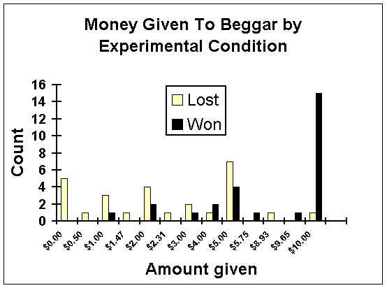
5> Next, I asked each of you how much of $10 you would give to a beggar.
6> What might a research hypothesis be for this study?
7> What are our two variables?
8> Which is our independent variable? How many levels does it have?
9> Which is our dependent or outcome variable?
10> Translate the research hypothesis into statistical hypotheses. What are these statistical hypotheses saying?
11> Set P value--or alpha--or the point at which we will reject the null hypothesis (that the difference we observe in the mean amount of money given between those who won and those who lost is simply due to chance).
12> Do z-test: (now technically we should do a two-sample t-test but the method is the same except for a slightly different denominator).
| Losing Group | Winning Group | ||
2.93 |
7.46 |
||
2.60 |
3.18 |
||
13.53 |
16.55 |
||
0.50 |
0.61 |
||
| =squareroot of (.502 | + .612) = | = 0.79 |
13> Reject null (for the correct t-test the p value was .05). Notice that the P for the z-value here is much smaller than a P of .05 (that would be a z of 1.96 for a two-tailed test) which is what is found with the correctly used t-test--the P we observe here is approximately .001 not the P of .05 for the t-test. So the z test, which is for big samples (100 at least in each group) is overestimating the rareness of the difference from what we expect to observe simply due to chance. That's because the denominator is too small--the SE's we estimated are biased, and should be corrected for the small sample size. But I use the two-sample z-test because that is what you have learned in class and we could walk through this step by step. Notice, however, that the math is the same whether the test is appropriate or not--knowing when to use a z-test or t-test is a decision you have to make, not a mindless handheld calculator.
14> Conclusions? Do you think the null hypothesis (the differences we observe between the two groups are simply due to chance) is plausible. Not according to our decision rule. So if the differences are not consistent with chance, that implies that the experience of winning or losing led students like you to be more or less generous toward the beggar. Do we know absolutely that that is true? No. But our results appear consistent with our alternative hypothesis.
15> Let’s talk about bias. How might bias have entered into our design? Do we expect our sample to be representative of our population? Was each group the same except for the experimental manipulation? What about those people who never give money to beggars? Did the experimental manipulation cause everyone to change what they did? Or did we just have to change the behavior of some people?
Analyzing the Results by a Chi-Square Analysis
We could also analyze our results with a chi-square test. Here, we would recode our data into categorical groups of giving the beggar nothing, something, or all the money you had. (We could also group it into giving nothing or giving something--deciding how to group outcomes takes judgment to do it in a way that communicates outcomes clearly to others---are there any other ways that make sense?)
Grouping our outcomes that way results in the following table that shows the counts for each cell and the marginal counts summing across either rows or columns:
| Gave: | Won Lottery | Lost Lottery | |
| Nothing | 0 | 5 | 5 |
| Something | 12 | 21 | 33 |
| All | 15 | 1 | 16 |
| 27 | 27 | 54 |
To do a chi-square test we:
1> Specify the research hypothesis
2> Translate that into two mutually exclusive statistical hypotheses, one of which we can evaluate--the null hypothesis. For the chi-square, the null hypothesis is that for all 6 cells here any departure of the count from what we would expect using only the information in the marginal counts is due solely to chance--that is the treatment effect is absolutely zero. We also have to decide what our decision rule will be. We decide to set our P, or alpha, conventionally at .05. So if the chi-square we obtain is likely to occur simply by chance alone 5% or less of the time, we will reject our null hypothesis.
3> Next we get ready to calculate the chi-square. To do so, we first create a new table with the expected cell frequencies, calculated using only the marginal counts as follows:
| Gave: | Lost Lottery | Won Lottery | |
| Nothing | (27*5)/54 = 2.5 | (27*5)/54 = 2.5 | 5 |
| Something | (27*33)/54 = 16.5 | (27*33)/54 = 16.5 | 33 |
| All | (27*16)/54 = 8.0 | (27*16)/54 = 8.0 | 16 |
| 27 | 27 | 54 |
Then we set up a table to keep track of our calculations:
| Condition | FO | FE | FO - FE | (FO - FE)2 | (FO - FE)2/FE |
| Gave nothing | |||||
| Won | 0 | 2.5 | -2.5 | 6.25 | 2.5 |
| Lost | 5 | 2.5 | 2.5 | 6.25 | 2.5 |
| Gave something | |||||
| Won | 12 | 16.5 | -4.5 | 20.25 | 1.23 |
| Lost | 21 | 16.5 | 4.5 | 20.25 | 1.23 |
| Gave all | |||||
| Won | 15 | 8.0 | 7.0 | 75.5 | 6.12 |
| Lost | 1 | 8.0 | -7.0 | 75.5 | 6.12 |
Chi 2 = |
19.70 |
In the F sub O column, we put the observed counts from the cells. In F sub E, we put the expected counts calculated using the marginal counts. Then going across the row, subtract the two, square the results, and divide by the F sub E for that row. This has the effect of weighting the deviation from what was expected by the size of the cell. The last step is to sum down the last column to get the chi-square value which is the sum of the weighted squared deviations.
4> Next, we have to figure the degrees of freedom for this analysis: (rows -1) * (columns - 1) = (3-2) * (2-1) = 2
5> Then, we go to the back of the book and look for the value in the table corresponding to 2 degrees of freedom and a 5% rejection rule. The value in the table is 5.99. So we compare our chi-square of 19.70 to this. Ours is bigger, which means that there is less than 5% chance that the deviation we are seeing is due to chance variation alone.
6> We make a decision--we reject our null hypothesis
7> That leaves only our alternative--that something more than chance is going on
8> So our last task is draw a conclusion--we accept our alternative hypothesis, and conclude that giving money to the beggar was associated with either winning or losing the lottery. Because this was an experiment we can make an even stronger statement about causation. Here goes: when people feel like they have just won the lottery they are more likely to give money to a beggar.
But you can also try your hand at other conclusions worded slightly differently. Here, too, is an important area for judgement. Good researchers draw well supported and intriguing conclusions from the studies they conduct.