Generalized Expectation Maximization [1]

This technical report describes the statistical method of expectation maximization (EM) for parameter estimation. Several of 1D, 2D, 3D and n-D examples are presented in this document. Applications of the EM method are also demonstrated in the case of mixture modeling using interactive Java applets in 1D (e.g., curve fitting), 2D (e.g., point clustering and classification) and 3D (e.g., brain tissue classification).

Table of Contents

1 Maximum Likelihood Estimation (MLE) 2

Example 1: Nornal(m,s²) 3

Example 2: Poisson(l) 3

2 General Expectation Maximization (GEM) Algorithms. 4

Application 1 (Missing Values) 4

Application 2 (Pattern Recognition) 4

Step 1 of EM (Expectation) 5

Step 2 of EM (Maximization) 6

3 EM Application: Finding Maximum Likelihood Mixture Densities Parameters via EM.. 6

4. Examples. 9

Example 1: Poisson(l) 9

Example 2: n-D Gaussian. 9

Example 3: 1D Distribution Mixture-Model-Fitting using EM.. 11

Example 4: 2D Point Clustering and Classification using EM.. 13

Example 5: 3D Brain Tissue Classification using EM and Mixture Modeling. 15

5. Online SOCR Demos. 15

6. References: 16

1 Maximum Likelihood Estimation (MLE)

First, let’s recall the definition of the maximum-likelihood estimation problem. We have a density function p (x | Q), that is governed by the set of parameters Q (e.g., p might be a Gaussian and Q could be the means (vector) and covariance (matrix)). We also have a data set of size N, supposedly drawn from this distribution with density p, i.e., X = {x₁, …, x_N}. That is, we assume that these data vectors are independent and identically distributed (IID) with distribution p . Therefore, the resulting joint density for the samples is:

is called the likelihood function of the parameters (Q) given the data, or just the likelihood. The likelihood is thought of as a function of the parameters (Q) where the data X is fixed (observed). In the maximum likelihood problem, our goal is to find a parameter vector Q that maximizes . In other words, we look for Q^* , where

Oftentimes we choose to maximize instead because it is analytically easier or computationally appealing.

Depending on the form of p (x | Q) this problem can be easy or hard. For example, if p (x | Q) is simply a single Gaussian distribution where the parameter vector Q=(m, s²), then we can solve the maximum likelihood problem of determining estimates (MLE) of m & s² by setting the partial derivatives of to zero (in fact, this is how the familiar formulas for the population mean and variance are obtained). For many problems, however, it is not possible to find such analytical expressions, and we must resort to more elaborate techniques (e.g., EM technique).

Example 1: Nornal(m,s²)

Suppose {X₁, …, X_n} IID N(m, s²), where m is unknown. We estimate m by: .

Example 2: Poisson(l)

Suppose {X₁, …, X_N} IID Poisson(l), where (the population mean, and standard deviation) l is unknown. Estimate l by:

2 General Expectation Maximization (GEM) Algorithms

The EM algorithm is one such technique, which allows estimating parameter vectors in the cases when such analytic solutions to the likelihood minimization are difficult or impossible. The EM algorithm [see references at the end] is a general method of finding the maximum-likelihood estimates of the parameters of an underlying distribution from a given data set when the data is incomplete or has missing values. There are two main applications of the EM algorithm.

Application 1 (Missing Values)

The first application of EM algorithm occurs when the data indeed has missing values, due to problems with or limitations of the observation process.

Application 2 (Pattern Recognition)

The second occurs when optimizing the likelihood function is analytically intractable, however, we still need to assume the likelihood function can be simplified by assuming the existence of and values for additional but missing (or hidden) parameters. This second application is more common in the computational pattern recognition community.

As before, we assume that data X is observed and is generated by some distribution. We call X the incomplete data. We assume that a complete data set exists Z=(X;Y) and also assume (or specify) a joint density function:

Recall that for each probability measure, P, P(A,B)=P(A|B)P(B) and hence, in terms of the conditional probability, P(A,B|C) = P(A|B,C)P(B|C). This joint density often times arises from the marginal density function and the assumption of hidden variables and parameter value guesses (e.g., mixture-densities, this example is coming up; and Baum-Welch algorithm). In other cases (e.g., missing data values in samples of a distribution), we must assume a joint relationship between the missing and observed values.

With this new density function, we can define a new likelihood function,

,

called the complete-data likelihood. Note that this function is in fact a random variable since the missing information Y is unknown, i.e., random, and presumably governed by an underlying distribution. That is, we can think of for some function , where X and Q are constant and Y is a random variable. The original likelihood is referred to as the incomplete-data likelihood function.

The Expectation Maximization algorithm then proceeds in two steps – expectation followed by its maximization.

Step 1 of EM (Expectation)

The EM algorithm needs to first find the expected value of the complete-data log-likelihood with respect to the unknown data Y given the observed data X and the current parameter estimates Qⁱ, the E-Step. Below we define the expectation of Q^(i-1), the second argument represents the parameters that we use to evaluate the expectation. The first argument Q simply indicates the parameter (vector) that ultimately will be optimized in an attempt to maximize the likelihood:

Q(Q, Q^(i-1))=E[Log p (X,Y | Q) | X, Q^(i-1)]. (1)

Where Q^(i-1) are the current parameters estimates that we used to evaluate the expectation and Q are the new parameters that we optimize to increase (maximize) Q. Note that the expression above is a conditional expectation w.r.t. (X & Q^(i-1)), i.e.,

E[ h(Y) | X=x] :=.

The key thing to understand is that X and Q^(i-1) are given constants, Q is a random variable that we wish to adjust/estimate, and Y is a random variable governed by the distribution f(Y |X,Q^(i-1)). The right side of equation (1) can therefore be expressed as:

(2)

The f(Y |X,Q^(i-1)) is the marginal distribution of the unobserved data (Y) and is dependent on: the observed data X, on the current parameters Q^(i-1), and Y is the space of values y can take on. In the best-case situations, this marginal distribution is a simple analytical expression of the assumed parameters Q^(i-1), and perhaps the observed data (X). In the worst-case scenario, this density might be very hard to obtain. In fact, sometimes the actually used density is:

f(y ,X | Q^(i-1))= f(y | X,Q^(i-1)) f(X | Q^(i-1)),

but this doesn’t effect subsequent steps since the extra factor, f(X | Q^(i-1)) is not dependent on Q.

As an analogy, suppose we have a function h( . ; . ) of two variables. Consider h( q ; Y ) where q is a constant and Y is a random variable governed by some distribution f_Y(y). Then

is now a deterministic function that could be maximized if desired, w.r.t. q. The evaluation of this expectation is called the E-step of the algorithm. Notice the meaning of the two arguments in the function Q(Q, Q^(i-1)). The first argument Q corresponds to the parameters that ultimately will be optimized in an attempt to maximize the likelihood. The second argument, Q^(i-1), corresponds to the parameters that we use to evaluate the expectation at each iteration (EàM à EàM à EàM à …).

Step 2 of EM (Maximization)

The second step (the M-step) of the EM algorithm is to maximize the expectation we computed in the first step. That is, we iteratively compute:

That is we maximize the expectation of the log-likelihood function. These two steps are repeated as necessary. Each iteration is guaranteed to increase the log-likelihood and the algorithm is guaranteed to converge to a local maximum of the likelihood function. There are many theoretical and empirical rate-of-convergence papers (see references below).

A modified form of the M-step is to, instead of maximizing the rather difficult function Q(Q, Q^(i-1)), we find some Q⁽ⁱ⁾ such that Q(Q⁽ⁱ⁾, Q^(i-1)) > Q(Q, Q^(i-1)). This form of the algorithm is called Generalized EM (GEM) and is also guaranteed to converge. This description of the GEM does not yield a direct computer implementation scheme (it’s not constructive (the coding algorithm is not explicit). This is the way, however, that the algorithm is presented in its most general form. The details of the steps required to compute the given quantities are very dependent on the particular application, so they are not discussed when the algorithm is presented in this abstract form, but rather detailed for each specific application.

3 EM Application: Finding Maximum Likelihood Mixture Densities Parameters via EM

The mixture-density parameter estimation problem is probably one of the most widely used applications of the EM algorithm in the computational pattern recognition community. In this case, we assume the following (mixture-density) model:

where the parameter vector is Q=(a₁, …, a_M ; q₁, …, q_M), where the mixture-model weights satisfy and each p_i is a density function parameterized, in general, by its own parameter vector q_i. In other words, we assume we have M component densities mixed together with M mixing coefficients a_i .

The incomplete-data log-likelihood expression for this density from the data X={x₁, …, x_N}, N = # Observations, is given by:

which is difficult to optimize because it contains the logarithm function of the sum [if the sum and the log were interchanged then optimizing the outside logarithm would have been equivalent to optimizing its argument – the sum – as the log function has always a positive derivative over its domain (0; )]. If we consider X as incomplete, however, and assume the existence of unobserved data items Y={y_i}_i=1^N, whose values inform us which component density “generated” each data item, the likelihood expression is significantly simplified. That is, if we assume that for each , and y_i=k if the i^th sample, x_i, was generated by the k^th mixture component p_k. If we know the values of Y, the likelihood becomes:

which, given a particular form of the component densities, can be optimized using a variety of techniques. The problem, of course, is that we do not know the values of Y. If we assume Y is a random vector, however, we can proceed. We first must derive an expression for the distribution of the unobserved (missing) data, Y. Let’s first guess at parameters for the mixture density, i.e., we guess that Q^g =(a₁^g, …, a_M^g ; q₁^g, …, q_M^g), are the appropriate parameters for the likelihood L(Q^g | X,Y). Given Q^g, we can compute p_j(x_i|q_j^g) for each i and j. In addition, the mixing parameters, a_i, can be though of as prior probabilities of each mixture component, that is a_i= p(component i). Therefore, using Bayes’s rule – P(Y_i|X_i)=P(X_i|Y_i)P(Y_i)/P(X_i), we can compute:

and therefore, , where y = (y₁, …, y_N) is an instance of the unobserved data independently drawn. When we now look at equation (2), we see that in this case we have obtained the desired marginal density (of Y), f(y | X,Q^(i-1)), by assuming the existence of the hidden variables and making a guess at the initial parameters of their distribution. In this case, equation (1) takes the specific form:

where . In this form, appears computationally challenging, however, it can be simplified, since for ,

This is because . Using equation (5), we can write equation (4) as:

Now, to maximize this expression, we can maximize independently F and Y, the terms containing a_l and q_l, since they are not related. To find the expression for a_l, which maximizes Q(Q,Q^(g)), we introduce the Lagrange multiplier l with the constraint that , and solve the following equation:

This yields:

Summing over l we get:

Therefore, l = -N , which yields that . This is how we determine the mixture parameters {a_l}, most of the time.

Now let us try to estimate the second part of the parameter vector Q=(a₁, …, a_M ; q₁, …, q_M), i.e., the distribution specific parameters (q₁, …, q_M). Clearly, these need to be estimated in a case by case manner, as different distributions have different number and type of parameters. We consider again a couple of cases that illustrate the basic strategy for estimating (q₁, …, q_M) using EM approaches. For some distributions, it will be possible to get analytic expressions for q_l directly, as functions of all other variables.

4. Examples

Example 1: Poisson(l)

Suppose that the mixture model in equation (3) involves Poisson(l_l) distributions, . Then the

Taking the derivatives w.r.t. l_l and setting these equal to zero yields,

Therefore, we have explicit expressions for iterative calculation of the estimates of the mixture parameters, Q=(a₁, …, a_M), and the Poisson distribution parameters, (q₁, …, q_M)=(l₁, …, l_M).

Example 2: n-D Gaussian

If we assume d-dimensional Gaussian component distributions with a mean vector m and covariance matrix S, i.e., q = (m; S) then the probability density function is

Then we may derive the update equations [equations (1), (4), (6)] for this specific distribution, we need to recall some results from matrix algebra. The trace of a square matrix tr(A) is equal to the sum of A’s diagonal elements. In 1D the trace of a scalar equals that scalar. Also, tr(A + B) = tr(A) + tr(B), and tr(AB) = tr(BA), which implies that . Also note that |A| indicates the determinant of the matrix A, and |A^-1|=1/|A|. Differentiation of a function of a matrix f(A) is accomplished by differentiating with respect to elements of that matrix. Therefore, we define df(A)/dA to be the matrix with (i,j)-th entry equal to [df(A)/da_i,j], where A=( a_i,j). This definition also applies taking derivatives with respect to a vector. First, d(x^TAx)/dx=(A+A^T)x. Second, it can be shown that when A is a symmetric matrix:

where A_i,j is the (i,j)-the cofactor of A. Given the above, we see that:

by the definition of the inverse of a matrix. Finally, it can be shown that dtr(AB)/dA = B + B^T-diag(B).

Now, for the d-dimensional Gaussian distribution example, if we take a log of equation (7), ignoring any constant terms (since they disappear after taking derivatives), and substituting into the right side of equation (6), we get:

Taking the derivative of equation (8) with respect to m_l and setting it equal to zero, we get:

which solving for m_l yields:

To find S_l, note that we can write equation (8) as:

where N_l,i = . In equation (9) we now take the derivative with respect to the matrix S_l^-1, and we obtain:

where N_l,i = , M_l,i = S_l – N_l,i and S = . To find the extreme values (maxima) of the , equation (9) we set the derivative to zero [equation (10)], i.e., 2S – diag(S) = 0. This implies that S=0 è So, we obtain an exact expression (variance-covariance matrix estimate, 1 l M) for S_l.

Summarizing, the estimates of the new parameters in terms of the old parameters (guessed parameters super-indexed by ^g, Q^g =(a₁^g, …, a_M^g ; q₁^g, …, q_M^g)) are as follows:

Note that the above equations (11) perform both the expectation step and the maximization step simultaneously. The algorithm proceeds by using the newly derived parameters as the guess for the next iteration.

Example 3: 1D Distribution Mixture-Model-Fitting using EM

These SOCR Activities demonstrate fitting a number of polynomial, distribution and spectral models to data: http://wiki.stat.ucla.edu/socr/index.php/SOCR_EduMaterials_ModelerActivities.

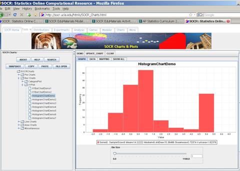
For instance, suppose we have a collection of 100 observations. The first 20 of these observations are included in the table below. A histogram of these observations is also shown below.

1	-2.51002
2	-2.51002
3	-1.5060121
4	-1.5060121
5	-1.5060121
6	-1.5060121
7	-1.5060121
8	-1.5060121
9	-1.5060121
10	-1.5060121
11	-1.5060121
12	-1.5060121
13	-1.5060121
14	-1.5060121
15	-1.5060121
16	-0.502004
17	-0.502004
18	-0.502004
19	-0.502004
20	-0.502004

These data was generated using SOCR Modeler:

http://socr.ucla.edu/htmls/SOCR_Modeler.html

http://wiki.stat.ucla.edu/socr/index.php/SOCR_EduMaterials_Activities_RNG

And the Histogram was obtained using SOCR Charts:

http://socr.ucla.edu/htmls/SOCR_Charts.html

http://wiki.stat.ucla.edu/socr/index.php/SOCR_EduMaterials_Activities_Histogram_Graphs

If these 100 random observations are copy-pasted in SOCR Modeler (http://socr.ucla.edu/htmls/SOCR_Modeler.html), we can fit in a mixture of 2-Normal Distributions to these data, as shown in the figure below. The quantitative results of this Em fit of 2 Normal distributions to these data is reported in the Results panel.

Mixture Model 0:

Weight =0.796875

Mean = 0.06890251005397123

Variance = 1.1959966055736866

Mixture Model 1:

Weight =0.203125

Mean = 4.518035888671875

Variance = 1.0

INTERSECTION POINT(S):

2.708939236914807

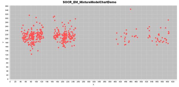
Example 4: 2D Point Clustering and Classification using EM

We can use the SOCR EM Chart, to enter real 2D data or simulate such data. The figure below shows the plot of knee pain data (courtesy of Colin Taylor, MD, TMT Medical).

· http://socr.ucla.edu/htmls/SOCR_Charts.html

· http://wiki.stat.ucla.edu/socr/index.php/SOCR_EduMaterials_Activities_2D_PointSegmentation_EM_Mixture

If we select four 2D Gaussian kernels, we can run iteratively the EM mixture-modeling algorithm to estimate the 4-clusters and finally classify the points in this knee-pain dataset, as shown in the figure below.

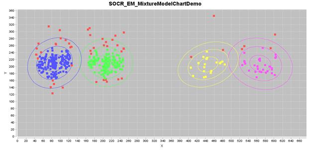
The estimated 2D Gaussian kernels are reported in the table below.

Kernel:1	Color[r=85,g=85,b=255]
mX = 12.109004237402402	mY = 117.82567907801044
sXX = 21.032925241685124	sXY = 78.7581941291246
sYX = 78.7581941291246	sYY = 24.09825818460926
weight = 0.430083268505667	likelihood = -10.208282817360221
Kernel:2	Color[r=85,g=255,b=85]
mX = 149.38436424342427	mY = 192.71749953677403
sXX = 20.76028543262703	sXY = -8.73565367620904
sYX = -8.73565367620904	sYY = 22.72742021102665
weight = 0.39741243015152933	likelihood = -10.208282817360221
Kernel:3	Color[r=255,g=255,b=85]
mX = 384.0858049258344	mY = 130.33122378944105
sXX = 23.636423858007923	sXY = 135.0559608391195
sYX = 135.0559608391195	sYY = 21.654643444147702
weight = 0.06547362085865455	likelihood = -10.208282817360221
Kernel:4	Color[r=255,g=85,b=255]
mX = 384.0858049258344	mY = 147.83898638544392
sXX = 25.080070954205347	sXY = -94.47319742216496
sYX = -94.47319742216496	sYY = 24.591327584325068
weight = 0.09143983449841454	likelihood = -10.208282817360221

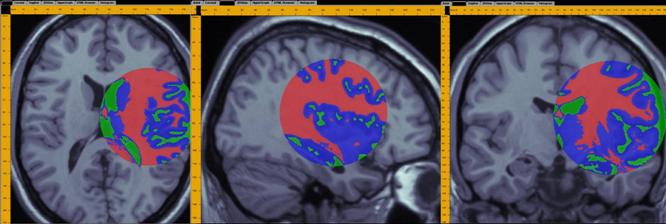
Example 5: 3D Brain Tissue Classification using EM and Mixture Modeling

A demonstration of a 3D data analysis using the SOCR EM Mixture model is included in the LONI Viz Manual (http://www.loni.ucla.edu/download/LOVE/LOVE_User_Guide.pdf). This example shows how 3D brain imaging data may be segmented into three tissue types (White Matter, Gray Matter and Cerebra-spinal Fluid). This is achieved by LONI Viz (Dinov et al., 2006) sending the segmentation tasks to SOCR and SOCR returning back the 3D segmented volumes, which are superimposed dynamically on top of the initial anatomical brain imaging data in real time. The figure below illustrates this functionality. Other external computational tools could also invoke SOCR statistical computing resources directly by using the SOCR JAR binaries (http://www.socr.ucla.edu/htmls/SOCR_Download.html) and the SOCR Documentation (http://www.socr.ucla.edu/docs).

5. Online SOCR Demos

· http://wiki.stat.ucla.edu/socr/index.php/AP_Statistics_Curriculum_2007_Estim_MOM_MLE

· http://wiki.stat.ucla.edu/socr/index.php/SOCR_EduMaterials_ModelerActivities

· http://socr.ucla.edu/htmls/SOCR_Modeler.html

· http://wiki.stat.ucla.edu/socr/index.php/SOCR_EduMaterials_Activities_2D_PointSegmentation_EM_Mixture

· http://wiki.stat.ucla.edu/socr/index.php/SOCR_EduMaterials_ModelerActivities_MixtureModel_1

6. References:

A.P.Dempster, N.M. Laird, and D.B. Rubin. Maximum-likelihood from incomplete data via the EM algorithm. J. Royal Statist. Soc. Ser. B., 39, 1977.

C. Bishop. Neural Networks for Pattern Recognition. Clarendon Press, Oxford, 1995.

J.A. Bilmes. A Gentle Tutorial of the EM Algorithm and its Application to Parameter Estimation for Gaussian Mixture and Hidden Markov Models. Department of Electrical Engineering and Computer Science, U.C. Berkeley, Berkeley, CA 94704, TR-97-021, April 1998.

Dinov ID, Valentino D, Shin BC, Konstantinidis F, Hu G, MacKenzie-Graham A, Lee EF, Shattuck DW, Ma J, Schwartz C and Toga AW. LONI Visualization Environment, Journal of Digital Imaging. Vol. 19, No. 2, 148-158, June 2006.

Z. Ghahramami and M. Jordan. Learning from incomplete data. Technical Report AI Lab Memo No. 1509, CBCL Paper No. 108, MIT AI Lab, August 1995.

M. Jordan and R. Jacobs. Hierarchical mixtures of experts and the EM algorithm. Neural Computation, 6:181–214, 1994.

M. Jordon and L. Xu. Convergence results for the EM approach to mixtures of experts architectures. Neural Networks, 8:1409–1431, 1996.

L. Rabiner and B.-H. Juang. Fundamentals of Speech Recognition. Prentice Hall Signal Processing Series, 1993.

R. Redner and H. Walker. Mixture densities, maximum likelihood and the EM algorithm. SIAM Review, 26(2), 1984.

C.F.J. Wu. On the convergence properties of the EM algorithm. The Annals of Statistics, 11(1):95–103, 1983.

L. Xu and M.I. Jordan. On convergence properties of the EM algorithm for Gaussian mixtures. Neural Computation, 8:129–151, 1996.

---

[1] This set of class notes is based on previous work by Bilmer, Bishop, Dempster, Ghahramami, Jordon, Rabiner, Redner, Wu and Xu see references at the end of the document.