iFRAME (inhomogeneous Filters Random Field And Maximum Entropy)

Experiment 2: Learning Mixture of Sparse FRAME Models for Clustering by Generative Boosting (with local shift)

clustering dataset

(1) code for sparse FRAME (2) code for active basis models (3) code for two-way EM (4) code for HOG + k-means

1. Experiment Setup

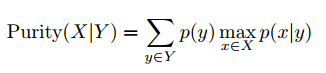
To evaluate the clustering quality, we introduce two metrics: conditional purity and conditional entropy. Given the underlying groundtruth category labels X (which is unknown to the algorithm) and the obtained cluster labels Y , the conditional purity is defined as the mean of the maximum category probabilities for (X, Y ),

and the conditional entropy is defined as,

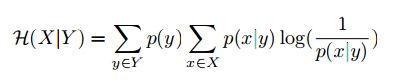
where both p(y) and p(x|y) are estimated on the training set, and we would expect higher purity and lower entropy for a better clustering algorithm.

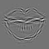
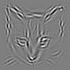
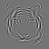
We compare clustering by sparse FRAME with (1) active basis model [1], (2) two-way EM [2], and (3) k-mean with HOG features. The methods are evaluated in terms of conditional purity and conditional entropy. All the results are obtained based on 5 repetitions. It can be seen that our method performs significantly better than other methods.

2. Parameter setting

Method 1: sparse FRAME by generative boosting

General Parameters: nOrient = 16; GaborScaleList=[1.4, 1, 0.7]; DoGScaleList =[]; LocationShiftLimit=3; OrientShiftLimit=1; interval=1; #Wavelet=300 or 350; isLocalNormalize=true;
Multiple Selection Parameters: nPartCol=5; nPartRow=5; part_sx=20; part_sy=20; gradient_threshold_scale=0.8
Gibbs Sampler Parameters: lambdaLearningRate = 0.1/sqrt(sigsq); 10x10 chains; sigsq=10; threshold_corrBB=0; lower_bound_rand = 0.001; upper_bound_rand = 0.999; c_val_list=-25:3:25
Clustering Parameters: rotateShiftLimit=3; numResolution = 2; scaleStepSize=0.1; numIterationEM=10; ratioDisplacementSUM2=0.45

Method 2: Active basis model

General Parameters: nOrient = 16; sizeTemplatex=100; sizeTemplatey=100; #basis=300; GaborSize=0.7; locationShiftLimit=4; orientShiftLimit=1;
Clustering Parameters: rotateShiftLimit=2; flipOrNot=1; numResolution = 5; #EM iteration = 7

Method 3: Two-way EM

General Parameters: sizeTemplatex=150; sizeTemplatey=150; cellsize=6x6; GaborSize=0.7; nOrient = 16; #Run=5

Method 4: k-mean with HOG

General Parameters: sizeTemplatex=100; sizeTemplatey=100; maxEMIter = 30; #HOG windows per bounding box =6x6; #histogram bins=9

3. Dataset

Profiles of UCLA mixture dataset for clustering tasks

	Description	# Clusters	Examples	# Images
Task 1	bull & cow	2		15/15
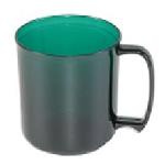
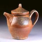
Task 2	cup & teapot	2		15/15
Task 3	plane & helicopter	2		15/15
Task 4	camel, elephant, & deer	3		15/15/15
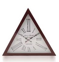Task 5	clocks (square, circle, triangle)	3		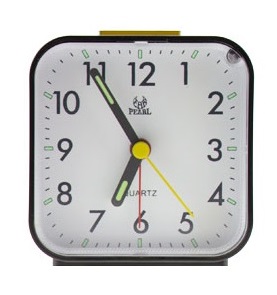15/15/15
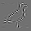
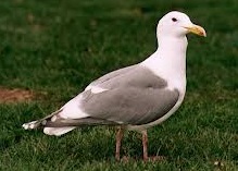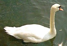Task 6	seagull, swan, & eagle	3		15/15/15
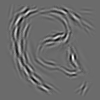
Task 7	eye, nose, mouth, & ear	4		15/15/15/15
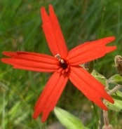
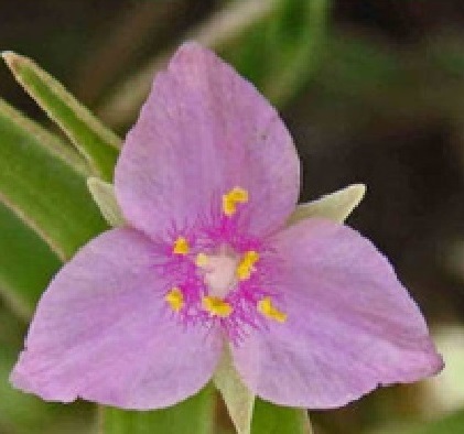
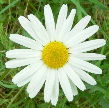
Task 8	flowers	4		15/15/15/15
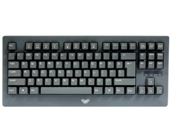
Task 9	keyboard, mouse, monitor, & mainframe	4		15/15/15/15
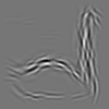
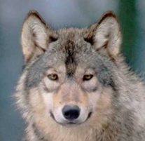
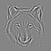
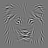
Task 10	tiger, lion, cat, deer, & wolf	5		15/15/15/15/15
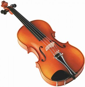
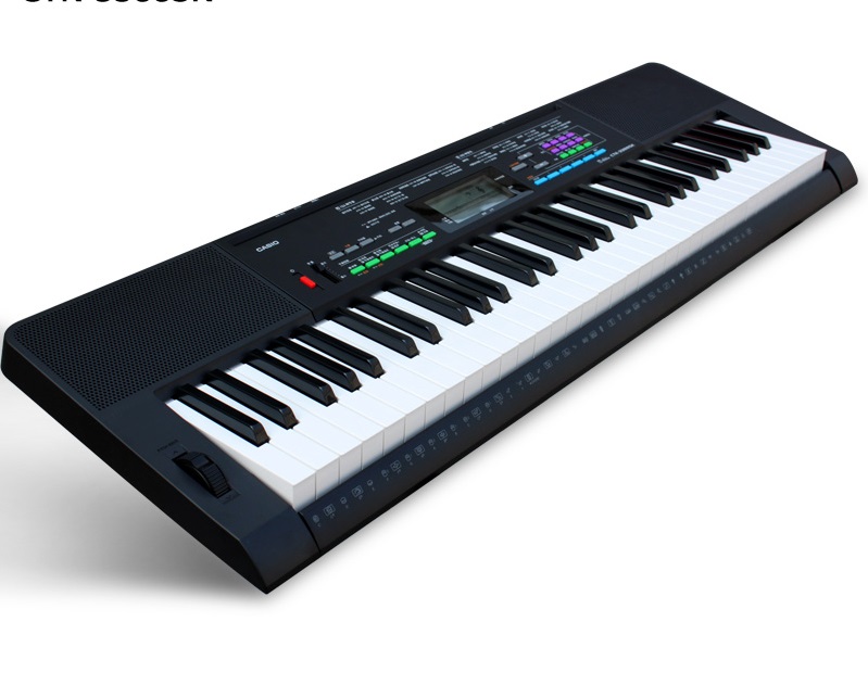
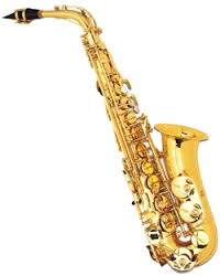
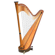Task 11	musical intrument	5		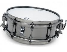15/15/15/15/15
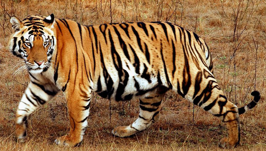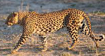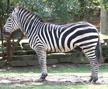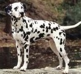Task 12	animal bodies	5		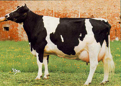15/15/15/15/15

4. Evaluation

5. Comparison

6. Visualization of some mixture models learned by sparse FRAME

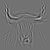
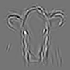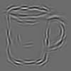
(Task 1) (Task 2) 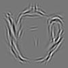(Task 6)

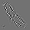
(Task 7) 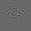(Task 10)

7. Reference

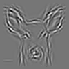
[1] Wu, Y. N., Si, Z., Gong, H., & Zhu, S. C. (2010). Learning active basis model for object detection and recognition. International journal of computer vision, 90(2), 198-235.
[2] Barbu, A., Wu, T., Wu, Y. N. (2014) Learning mixtures of Bernoulli templates by two-round EM with performance guarantee. Electronic Journal of Statistics, 8, 3004-3030.