Stats 110A, Fall 99 Midterm
Name:
SID:
Show all work. The points for each problem are shown in parentheses besides each part.
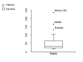
1. Below is a boxplot showing the average cost of a BigMac in 45 different cities from around the world. (Ignore the "options" and "zero line" symbols.) Cost is measured in the minimum average minutes of labor required to purchase a BigMac.
a) (2) Half of the cities in this sample must work for about how many minutes or less in order to buy a Big Mac?
This is the middle line in the box: close to 30.
b) (4) Is the average cost likely to be greater than, less than, or about equal to the median cost, and why?
The average is likely to be greater than the median, because the outliers, and the skewed shape of the distribution, pull the average up.
(Number 1 continued)
c) (5) Here are some observations from this data. Make a stem& leaf plot:
31 33 98 131 31 105 103 18 39 29 22 22 21 40 24 27 35 57
Stems are the digits 1,2,3,4,5,6,7,8,9,10. I can't make a s & l plot for HTML, so you'll have to come and look at the key if you have questions.
2. From the same data set as number 1 comes this graph, which graphs average costs of a Big Mac (in terms of minutes of labor ) and the average engineer's salary (in thousands of U.S. dollars) for these 75 cities.
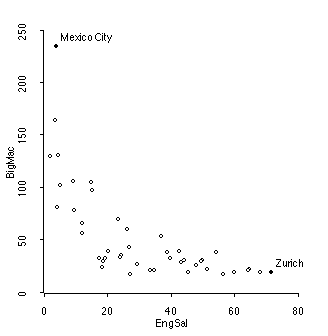
a. (5) Describe the relationship between average engineers' salaries and the cost of Big Macs.
The trend is negative, which means that cities with higher average engineers' salaries also have "cheaper" average Big Macs. Note that it is not correct to say that increasing engineering salaries will decrease the cost of Big Macs, because the data do not have any examples in which salaries were changed. Also, you need to be as precise as possible. The data are not comparing engineers, but are instead comparing cities.
The trend is non-linear (maybe exponential?) and moderately strong.
(Number 2 continued)
Here are some summary statistics for these two variables.
Data set = Mac, Summary Statistics
Variable N Average Std. Dev Minimum Median Maximum
BigMac 45 53.289 45.082 18. 34. 235.
EngSal 45 31.016 19.739 1.9 26.9 71.7
Data set = Mac, Sample Correlations
BigMac 1.0000 -0.6833
EngSal -0.6833 1.0000
BigMac EngSal
b. (5) Find the regression line
b = r*s_y/s_x = -0.6833*45.082/19.739 = -1.56
a = ybar = bxbar = 53.289 - (-1.56) * 31.016 = 101.69
yhat = 101.69 - 1.56x
c. (2) Graph the regression line on the scatterplot on the last page. Show details.
You're on your own for this one, too.
d. (5) Interpret the regression line. Comment on whether you think the line is a "good" summary or a poor summary of the trend.
You should note that its a very poor fit. Most points are below the regression line, particularly in the middle range of the x-variable. The relation is NOT linear, and so normal indicators like r or r-squared are not too helpful.
None-the-less, if we are to interpret the coefficients, the slope indicates that cities with average engineers' salaries 1000 higher, have average cost of Big Mac's 1.56 fewer minutes of labor, on average. The intercept tells us nothing.
3. A Statistics professor wants to determine whether a new computer lab assists student learning. He makes up a group of exercises to be done on the computer, and announces that these are optional exercises to be completed during the quarter. At the end of the quarter, he notices that 10 students did all of the exercises, 8 students did some of the exercises, and 20 students did none of the exercises. He also noted that the average score on the final exam for the students who did all exercises was about 10 points higher than those who did only some of them. And the students who did only some of the exercises scored about 5 points higher, on average, than those who did none.
a) (5) Is this an observational study or a controlled study? Explain.
This is an observational study because the subjects (the students) themselves chose which group to belong to: the "treatment" group (do all computer excersies), the "partial treatment group" do some of the problems, and the "control" group (do none of the problems.
b) (5) If you said it was an observational study, what would you change, add, or delete, to make this a controlled study? If you said it was a controlled study, answer these questions: Which of these populations would you feel comfortable extending these results to and why? All students in this class? All students at the professor's university? All students at all universities in the U.S.? Explain your answer for each of these populations.
The reason that this is an observational study is because the subjects chose their treatment themselves. To make it a controlled study, therefore, you need to simply undo this: have the prorfessor assign students to groups. These groups can be like above (all, some, or none of the computer problems), or maybe just have two groups: all or none.
Many of you mentioned that the groups should be randomly assigned. Also, that there should be a "placebo" (although its difficult to imagine what this might be), and also that the professor shouldn't know which students were in which group, particularly when it came time to grade the final. All of these points are good ones, and in a well-designed study they would be done to the extent possible. However, they are not necessary to make us classify the study as "controlled". All that is necessary is that the subjects be assigned to treatment groups by the researchers. (This doesn't mean, of course, that it will be a good controlled study. Merely controlled.)
c) (5) The professor concluded that the computer improved performance on the final exam. Do you agree or disagree? Explain.
You should disagree. There are many other ways of explaining the outcome. For example, students who were motivated and interested in the topic are probably more likely to do well overall, and also more likely to take the time to do extra computer-based problems. In short, the structure of the study does not eliminate any number of possible confounding factors.
4. (2) A fair coin is flipped 10 times. Which of the following outcomes, if any, is most likely, and why?
HTTHHHTHTH
HTHTHTHTHT
This is deliberately a tricky question, and it helps point out one of the many places in which our intuition about probability fails us. The answer is that both sequences have the same probability of occurring. Because coin flips are independent, the probability of the first is
P( first is H AND second is T AND second is T AND ....last is H) = .5 ^ 10
And the second is P(First is H AND second is T AND third is H....) = .5^10
The second one "looks" less random because we see a pattern in it. However, it is just as likely (or unlikely) to occur as any other arbitrary sequence.
5. (5) A major concern in designing surveys is choosing an appropriate sample size. For example, a company is test marketing a certain product. They take a random sample of 50 people and ask them to rate the product as follows: 1 == "would never buy this" 2 =="might buy this if it cost less than $20" 3== "might buy this if it cost less than $10".
The company president has decided to go ahead and sell the product if at least 25% of the market would answer with a 2 or 3. "But", he says to his statistician, "Let's say for the sake of argument that 75% of the market would answer '1', 5% would answer '2', and 20% would answer '3'. What's the probability that after our survey, we'll mistakenly conclude that LESS than 25% of the market will answer with a 2 or 3?" Design a simulation that would find the experimental probability that, with a population like the president suggests, a survey of 50 people will result in fewer than 25% people responding with a "2" or "3". List each step and justify.
I. The Model is a box with 100 tickets. 25 of the tickets are "1"s and represent a response of 2 or 3 on the survey. The remaining 75 tickets are "0"s and represent the response of 1 on the survey. This captures the key probability characteristic that the president is proposing: there is now a 25% that any ticket chosen will represent a 2 or 3, just like the proposed population.
II. Define a Trial: Draw 50 tickets with replacement. This simulates the act of surveying 50 people.
III. Define a successful trial: A successful trial is one in less than 25% of the tickets are "1"s. So the trial is a success if the sum of the tickets is 12 or fewer.
IV. Repeat this many (N) times.
V. The probability we are interested in is, experimentally, the number of successes over N.
TURN PAGE FOR LAST QUESTION