Midterm 2

Name:

ID:

Tables are included in the back to assist you. You must show your work for full credit.

1. What is a "healthy" body temperature for adults? Traditionally, 98.6 degrees Farenheit was believed to be the mean adult body temperature, and if your temperature was too far above or below this, then it was a sign of illness. HOWEVER, recent research suggests that the true mean body temperature might be less than 98.6.

Here are body temperatures taken from a random sample of 21 healthy adults in a study:

98.0, 99.0 98.4 98.4 98.8 97.6 98.0 99.5 98.6 97.2 98.5 98.8 98.0 98.6 98.5 98.6 97.9 98.8 98.7 97.9 98.4

Below are summary statistics for these data computed using DataDesk.

Summary of temp

No Selector

Percentile 25

Count 21

Sum 2066.20

Mean 98.3905

Median 98.5000

StdDev 0.516628

Min 97.2000

Max 99.5000

IntQRange 0.725000

Lower ith %tile 98

Upper ith %tile 98.7250

a) (5) Assume that the distribution of body temperatures for healthy adults is normally distributed with mean 98.6 and SD 0.52 degrees. What is the probability that a randomly selected adult will have a temperature less than 98.4 degrees?

Let X represent the temperature of a randomly selected, healthy adult. Assuming, as the problem tells us to, that X is N(98.6, 0.52), P(X < 98.4) = P(Z < (98.4 - 98.6)/.52) = P(Z < -.385) = .3520 (or .3483, depending on how you rounded off.)

b) (5) Assume that the distribution of body temperatures for healthy adults is normally distributed with mean 98.6 and SD 0.52 degrees. We randomly select 21 healthy adults and compute their average temperature. Find the probability that this average is less than 98.4.

Now Xbar is N(98.6, .52/sqrt(21)) or N(98.6, 0.11347330). So P(Xbar < 98.4) =

P(Z < -.2/.1134733) = P(Z < -1.76) = 0.0392.

Note that this probability is exact. If X1, X2,...Xn are N(98.6, .52), then Xbar is exactly N(98.6, .52/sqrt(21)).

c) (5) Assume that the distribution of body temperatures is normal, but the mean and SD is unknown. Find a 95% confidence interval for the mean body temperature of a healthy adult, based on these data. Show all work.

The true SD is unknown, but s = 0.516628 is our estimate of it, based on our sample. Likewise, the true mean is unknown, but Xbar = 98.3905 is our estimate based on our sample. The 95% CI is

Xbar +- t* s/sqrt(21)

where t* is the number that cuts off 2.5% in the upper tail in a t-distribution with n-1 = 20 degrees of freedom. So from Table F, t* = 2.09.

98.3905 +- 2.09*.1134733

98.3905 +- 0.23715920

(98.153341, 98.627659)

is 95% Confidence interval.

MORE ON NEXT PAGE

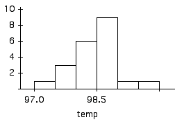
d) A simulation study used a computer to draw a sample of size 16 from a normal distribution with mean 98.6 and SD 0.5166. An average was computed. This was repeated 500 times. The results are in the histogram below. (Hint: the histogram uses the left-hand rule: an observation with value x is included in the bin [a,b) if a <= x < b. So the first bin contains those values greater than or equal to 98.275, but strictly less than 98.3.)

NOTE: This problem contains a typo. The "16" should have been a "21", which was the value used in the actual simulation, and is the correct value to use if this simulation is to represent the actual study. However, if you interpreted the histogram below to represent samples of size 16, it would not affect your conclusion for part (ii) (or part i for that matter) because if this were a histogram based on sample size 16, then the histogram for sample size 21 would be even narrow, and the probability you got in part i would be even smaller.

i) (2) Use this histogram to find the experimental probability that the average of a sample of 21 people will be less than 98.4.

There are 16 trials (out of 500) in which the average was less than 98.4, so this represents an experimental probability of 3.2% (Compare this to part b, above, in which the theoretical value for the same thing was about 3.9%.)

ii) (5) Do you think this is evidence for, or against, the hypothesis that the true mean temperature is 98.6? Explain.

This is evidence against the hypothesis that the true mean temp. is 98.6. The simulated data come from a distribution in which the mean really is 98.6. We see that, in such a context, we only get averages of 98.4 about 3% of the time. This suggests that either the true mean is less than 98.6 or the sample of 21 people we observed are so unusual that we'll only see such things 3% of the time.

MORE

2. A large box sits in the middle of a room occupied by 100 statisticians. Each statistician takes a random sample of 16 tickets from the box (with replacement), and uses the values on these tickets to estimate the mean value of all of the tickets in the box. Each statistician computes an 80% confidence interval for the mean.

a) (5) Find the probability that of the 100 confidence intervals produced, exactly 10 fail to include the mean of all of the tickets in the box.

The probability that a single confidence interval covers the true mean is 80%. Let X represent the number of statisticians out of 100 who have a "bad" confidence interval. The X is a binomial random variable with n = 100 and p = .20. Why? We have 100 indpt, trials, the outcome of each trial is "success" ( the CI fails to cover the mean) and "failure" (the CI does cover the true mean), the probability of success is the same for each trial : .20.

So P(X = 10) = "100 choose 10" * .2^10 * .8 * 90

b) (5) Use the normal approximation to find the approximate probability that at at most 10 statisticians will compute confidence intervals that fail to include the mean of all of the tickets in the box.

X is really binomial with n=100, and p = .2. So E(X) = np = 20 and SD(X) = sqrt(np(1-p)) = 4.

You can check that both np and n(1-p) are bigger than 10, so the normal approximation will be a good one.

So we can approximate the pdf of X as being N(20, 4)

P(X < 10) =(approx) P(Z < (10-20)/4) = P(Z < -10/4) = P(Z < -2.5) = 0.0062

3. The Federal Highway Commission estimates annual household vehicle miles travelled (VMT). Independent samples of 14 southern households and 15 midwestern households yielded the following data. (The data are sorted within each group from smallest to largest.) The units are thousands of miles per year.

Midwest: 9.6, 10.8, 11.2, 12.9, 14.6, 15.1,16.2,16.6, 16.6, 17.3, 18.3, 18.6, 20.3, 20.9, 24.4

South: 9.3, 11.5, 12.2, 15.8, 16.0, 17.5, 18.0, 18.2, 19.2, 20.1, 20.2, 22.2, 22.8, 24.6

The combined median, that is, the median of both sets of observations combined, is 17.3.

It is hypothesized that people in the South drive farther, in general, than people in the Midwest. To address this issue, answer the following questions:

NOTE: This was the one with the big typo. I have changed this version to be "correct". (The mistake was that where I typed "midwest", I meant to type "south", and vice-versa.) You could do the problem, still, with the mistake in place, and full credit was given if this is what you did.

a) (5) Do you think the typical VMT for the Midwest is less than the South, or do you think they are about the same? Give evidence from the data (descriptive statistics) to support your point of view.

One piece of evidence (you might have chosen others): The midwest has only 5/15 observations greater than the "combined" median of 17.3, while the South has 9/14.

b) (22) Design a 6-step simulation to perform a median test. Include:

i) (5) Model for the null hypothesis.

A box will 29 tickets each with one of the values from above on it.

ii) (5) Definition of a trial

A trial consists of pulling out 14 tickets, without replacement, that represent the "south".

iii) (5) Definition of a successful trial

A trial is "successful" if 9 or more tickets are above 17.3. The null hypothesis says that such occurrences are quite common and due only to chance. The "alternative" is that they are strong evidence that the South drives more.

iv) Repeat 100 times

v) (2) Describe how to calculate the experimental probability of success

Calculate the total number of successes divided by 100.

vi) (5) Explain how you would decide whether or not to reject the null hypothesis, and why.

If this probability was big, then the null hypothesis is right: such differences do occur by chance fairly frequently. If the probability is small, say less than 5%, then while it is true that we might see 9/14 above the median just by chance alone, this doesn't happen very often, and so this supports the alternative and we should reject the null hypothesis.