Due Friday, April 27
3.2, p. 117
5
3.3
2,5,6
3.4
4
Chapter Review (p. 142)
1,2
A. (From Freedman, Pisani, & Purves). In a study of 1993 Math SAT scores, the Educational Testing Service computed the average score for each of the 51 states (including D.C.), and the percentage of the high-school seniors in that state
who took the test. The correlation between these two variables was equal to -0.86.
a) True or False : test scores tend to be lower in the states where a higher percentage of the students take the test. If true, how do you explain this? If false, what accounts for the negative correlation?
b) In New York, the average score was only 471. But in Wyoming, the average was 507. True or false, and explain: the data show that on average, the schools in Wyoming are doing a better job at
teaching matht than the schoolf in New York.
B. (From Moore & McCabe) Researchers studying acid rain measured the acidity of precipitation in an isoilated wilderness are in Colorado for 150 consecutive weeks in the years 1975 to 1978. The acidity of a solution is
measured by pH, with lower pH values indicating that the solution is more acid. The acid rain researchers observed a linear patern over time. They reported that the least-squares line
pH = 5.43 - (0.0053)* weeks
fit the data well.
a) Draw a graph of this line.
b) According to the fitted line, what was the pH at the beginning of the study (weeks = 1)? At the end (weeks = 150)?
c) What is the slope of the fitted line? Expalin clearly what this slope says about the change in the pH of the precipitaiton in this wilderness area.
C. (From Moore & McCabe.) A study of erosion produced the following
data on the rate (in liters per second) at which water flows across a soil
test bed and the weight (in kilograms) of soil washed away:
| Flow | Soil |
| .31 | .82 |
| 1.26 | 2.18 |
| .85 | 1.95 |
| 2.47 | 3.01 |
| 3.75 | 6.07 |
a) Plot the data
b) Find the equation of the least squares line. Superimpose it on your graph.
c) Interpret the line (the slope and intercept).
d) How much soil should we expect to be washed away if the flow rate
is 2.00?
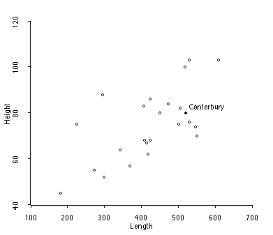
D. The data below graphs the nave length and the nave height for several cathedrals in England. Here is a picture of the nave at Canterbury Cathedral. (Read the Canterbury Tales for a point of reference. Or Death in the Cathedral.)


Here's some summary statistics:
| Variable | N | Average | St. Deviation | Minimm | Median | Maximum |
| Height | 25 | 75.16 | 15.01 | 45 | 75 | 103 |
| Length | 25 | 429.44 | 110.34 | 182. | 425 | 611 |
The correlation is r = 0.64.
a) Find the least squares line.
b) Plot the line on the graph above.
c) What is a typical nave height if the length is 500 feet? Is Canterbury typical in this sense?
d) Interpret the slope of the line.
e) In your opinion, is the line a good fit to these data? How would
you tell?
E. Runners are concerned about their form when racing. One measure of
form is the stride rate, the number of steps taken per second. As running
speed increases, the stride rate should also increase. In a study of 21
of the best American female runners, researchers measured the stride rate
for different speeds. The following table gives the speeds (in feet per
second) and the mean stride rates for these runners. (Data from R.C. Nelson,
C.M. Brooks, and N.L. Pike, "Biomechanical comparison of male and female
distance runners," in P. Milvy (ed.), The Marathon: Physiological, Medical,
Epidemiological, and Psychological Studies, New York Academy of Sciences,
1977, pp. 793-807.) Problem from Moore & McCabe, Introduction to the
Practice of Statistics, Third Ed.
| Speed | 15.86 | 16.88 | 17.5 | 18.62 | 19.97 | 21.06 | 22.11 |
| Stride Rate | 3.05 | 3.12 | 3.17 | 3.25 | 3.36 | 3.46 | 3.55 |
a) Plot the data with speed on the x axis and stride rate on the y axis. Does a striaght line adequately describe these data?
b) Find the equation of the regression line of stride rate on speed. Draw this line on your plot.
c) For each of the speeds given, obtain the predicted value and the residual. Verify that the residuals add to 0.
d) Plot the residuals against speed. Describe the pattern. What does
the plot indicate about the adequacy of the linear fit? Are there any potentially
influential observations? Can you plot the residuals against the time at
which the observations were made?
F. From your textbookk, Section 4.1, p. 159:
2, 4