Textbook Example 3
More about the Central Limit Theorem
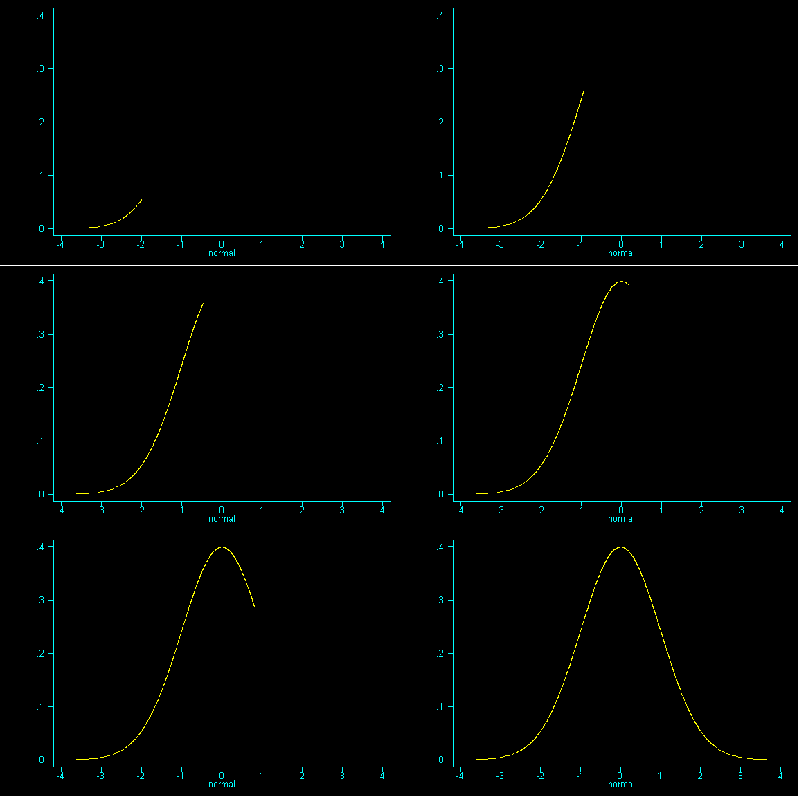
Statement of the Theorem
The central limit theorem and the law of large numbers are the two fundamental theorems of probability. The central limit theorem states that the distribution of the sum of a large number of independent, identically distributed random variables will be approximately normal, regardless of the underlying distribution. The existence of the central limit theorem is crucial to statistics, it is the reason that many statistical procedures work.
Perhaps it would help to restate the idea italicized above:
Data generated by repeatable random processes and subject to many small and unrelated random effects will be approximately normally distributed.
In Chapter 17.3, we observe that the SUM of many repetitions of some given number of draws will be normally distributed. The reason why it "works" is explained in Chapter 18.
One nice result is the probability histogram (or sampling distribution) of the sum becomes increasingly bell-shaped, as the sample size increases, regardless of the shape of the underlying population (i.e. the pattern of tickets in the box).
This fact is of fundamental importance, because it means that we can approximate the distribution of certain statistics, even if we know very little about the population and its parameters.
Of course, the term "large" is relative. Roughly, the more "abnormal" the basic distribution, the larger your sample size must be for normal approximations to work well. The rule of thumb is that a sample size n of at least 30 will suffice; your textbook prefers a sample size n of at least 100, although for many distributions smaller n will do.
To better understand the Central Limit Theorem, let's watch it in action. Here is a population, it is strongly RIGHT skewed:
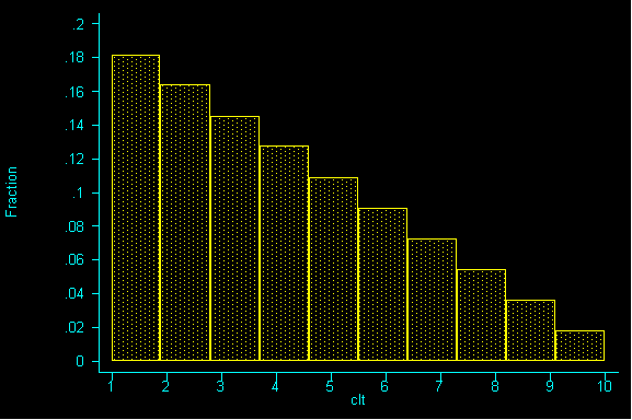
Here are its parameters: average=4, standard deviation=2.472
Now, PRETEND you do not know what the population looks like and PRETEND you did not know the parameters. But suppose, you wanted to know the population average.
A real life situation might be this: we don't know if the American population is earning more money this year than last year, but we would like to know it's total (sum). Once we know the sum, we can divide by the total number of items that went into the calculation of that sum to get a mean.
Back to our right skewed example: suppose we were to draw a sample of size 1 and then draw a second sample of size 1, and then a third sample of size 1 and a fourth sample of size 1, etc. until we had all possible samples of size 1.
QUESTION 1: Suppose our samples really were of size 1, what would be the expected value and standard error for the sum?
If we drew enough samples, we'd have a replica of our population...but it's not very quick way to get information. We can see it simulated below:
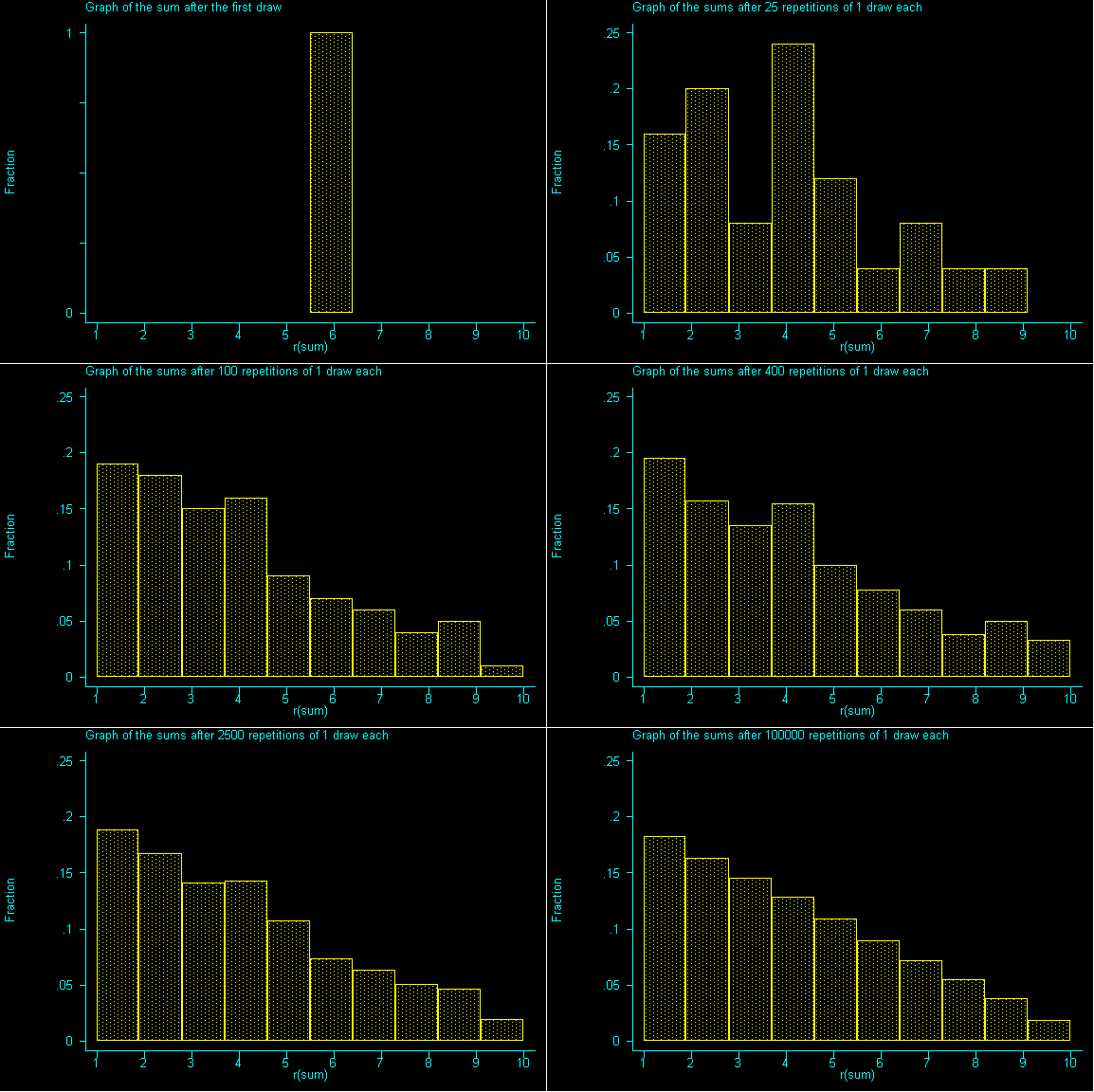
For this class, 100,000 repetitions is effectively infinite.
What happens when we increase the sample size to 9? And drew sample after sample of size 9 until we had all possible samples and then graphed the resulting sums.
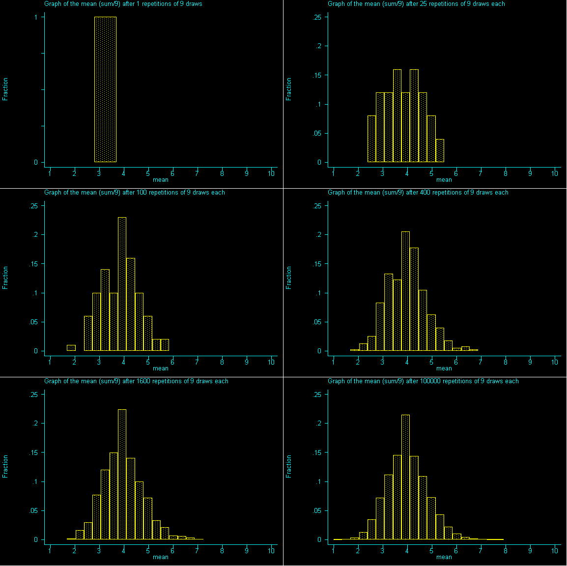
QUESTION 2: Now with samples of size 9, what would be the expected value and standard error for the sum? Then, divide the expected value of the sum by the sample size to get the expected value for the mean. Also, divide the standard error for the sum by sample size to get the standard error for the mean.
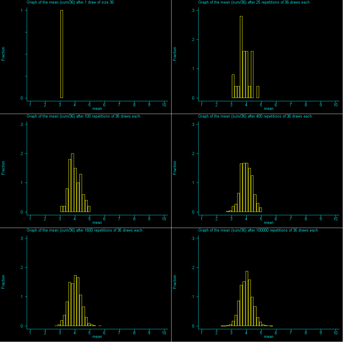
QUESTION 3: Now with samples of size 36, what would be the expected value and standard error for the sum? If you've done question 2, please calculate the expected value for the mean and the standard error for the mean.
QUESTION 4: As we move from samples of size 1 to 9 to 36, what do you notice about the expected sum? How is it changing? How is the the expected value of the mean changing? How are the standard errors for the sum and for the mean changing?
QUESTION 5: Looking at the graph of samples of size 36, what value is the probability histogram trying to center around?
If you guessed -- the expected value (or an even better guess) -- the population mean of 4 (a parameter), you are right.
What you should realize after working through this example is that the mean of the probability histogram (sampling distribution) is the same as the mean of the population.
QUESTION 6: After thinking about question 5 and understanding that the population mean is the same as the mean of the probability histogram (or sampling distribution). The "spread" of the Probability Histogram or Sampling Distribution is actually called the (fill in the blank)