NAME:
ID:
Write neatly and clearly. Explain your answers when necessary. Equations and tables are provided in a separate packet. All questions are worth 5 points unless otherwise indicated.
A. Were there differences in salary between men and women at a small midwestern university in the early 80's? Refer to the data on the following pages to answer these two questions. Additional blank pages are provided after the data.
1. What are your initial impressions as to whether there is a difference in salary based on gender? What evidence did you use to reach this conclusion?
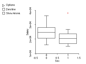
Based on the boxplots, it looks as if women make less. The median women's salary is quite a bit less than the men's (in fact, almost the same as the first quartile. So half of the women make less than 25 percent of the men.) Interestingly, there is one outlier: a woman who makes more than everyone else.
2. Carry out a formal statistical test to see if there are differences between men's and women's salaries. Various tables are at the end to help you. If it makes things easier, you may assume that the variance in salaries is the same for both groups. Your work should follow this format: (5 pts each) (Blank page follows for additional work.)
a) State your assumptions
Assume that salaries are normally distributed and independently assigned. (This is probably not a good assumption!) We'll assume that the variance of salaries in each group (M and W) are equal and unknown.
b) State the significance level you are testing at.
5%, although any significance level is fine. At least as far as this midterm is concerned.
c) State the null and alternative hypothesis
The null is that mean(men) = mean(women). The alternative is that mean(women) < mean(men).
d) Calculate the appropriate test statistic or confidence interval.
We'll use Xbar - Ybar to estimate the difference in the means. (The men's salaries are the X's, the women's the Y's.) The standard error is sigma times the square-root of (1/n) + (1/m), where n and m are the numbers of men and women, respectively. Sigma is the unknown SD of the salaries, and we can estimate this by pooling the observations to calculate the pooled sample variance. (This formula was given with the test.) I'll try to reproduce it here, but it's hard to do in HTML.
sp^2 = (n-1)*sx^2 + (m-2)*sy^2 divided by (n+m-2) = ((37 * 5646.409^2) + 13*(6151.8731^2))/50
The square-root of this is 5782.08 = sp. So the SE is
sqrt(1/38 + 1/14) * 5782.08 = 1807.71.
So our test statistic is (24696.789 - 21357.143)/1807.71
= 1.84745
e) Do you conclude that this university was taking gender into account when making salary decisions?
Yes. This test statistic follows a t-distribution with n+m-2 = 50 degrees of freedom. This is closely approximated by a normal distribution, and so to reject the null hypothesis that the mean salary for men is equal to the mean salary for women, in favor of the (one-sided) hypothesis that the mean men's salary is greater than the mean women's salry, requires a test statistic exceeding 1.654.
Note that had you stated that your alternative hypothesis was that men make a different salary than women, on average, then you would have done a two-sided test and rejected the null hypothesis if your test statistic exceeded 1.96. In this case, you would have concluded that there was no evidence of a difference between the two group means, and therefore no evidence that gender played a role in salaries.
Another way to do this is to calculate an approximate
p-value using the normal table. A one-sided p-value for 1.85 is 1-.9678
= .0322. At a 5% significance level, you would reject and say that there
was sufficient evidence to conclude that women, on average, made less then
men. The two-sided p-value is 0.0644. At the 5% level, you would conclude
that there was no evidence that the mean salary of men differed from the
mean salary of women.
Which test, the one-sided or the two-sided is better? In real-life, it is probably best to take the more conservative approach. In this case, it creates some controversy, and so you must be able to back up your choice of a one-sided hypothesis. In my opinion, the one-sided test is a little more difficult to sell, because it doesn't refute what would be the college's main argument: the difference is due to chance, and could just as easily gone the other way.
f) How would you use the data to check the assumptions you made? (Some might be uncheckable.)
The main checkable assumption here is that of normality and the equal variances. The normality assumption can be made by separate normal probability plots of the salaries of the two groups. The points in each plot should fall along a straight line. The equal variances assumption can be roughly eye-balled by looking at the box-plots, but it is much better to do the F-test (sy/sx) and check. Better yet, also present the version of the test that does not require this assumption (in this version, you estimate the degrees of freedom from the data and get an approximate t-test) and see whether they agree with your previous results. If the conclusions affirm your first results, then there is no need to argue about whether the assumption holds. If not, things get interesting, and you might want to consider accepting the more conservative conclusion (which is produced by the test that does not assume equal variances.)
DATA for Question A
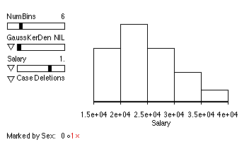
(Men are coded as 0, Women as 1. The last item below, q(0.5,) is the median. In all plots, the x's are women, the o's are men.)
Table of Salary: Count
Column variable: Sex
0 1
|--------
| 38 14
Table of Salary: Mean
Column variable: Sex
0 1
|--------------------
| 24696.789 21357.143
Table of Salary: SD
Column variable: Sex
0 1
|--------------------
| 5646.409 6151.8731
Table of Salary: Minimum
Column variable: Sex
0 1
|------------
| 16094 15000
Table of Salary: Maximum
Column variable: Sex
0 1
|------------
| 36350 38045
(Continued)
Table of Salary: q(0.5)
Column variable: Sex
0 1
|------------
| 24746 20495

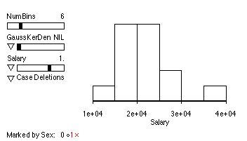 Women (above)
Men (below):
TURN THE PAGE FOR THE NEXT QUESTION.
B. A factor that might be expected to play a role in salary decisions is the years since the last degree was earned. This is one way of measuring experience. (Another way is to measure the years at the university, but frequently universities hire people from other universities who might make high salaries.) The data on the following pages relate salary to the years since last degree earned (YSDegree). Use these data to answer these six questions:
1. (10 pts) Describe the relationship between years since degree and salary. What does the regression line tell us about this relationship?
Those who earned their degree most recently tend to make less than those who earned their degree a while ago. Of course, there are many exceptions to this. The trend seems to be linear, or at least there are no strong indications otherwise. The constant of the regression line suggests that those hired for the first time after earning their degree make an average of $17402.30 at this institution. The slope suggests that those with a year's more time since earning their degree make, on average, $390.65 more. Note that this does NOT mean that each year individual faculty's salaries increase. In fact, they might go up at regular intervals, or they might not go up at all! This data set contains no information tracking individuals' salaries over time, and so for all we know, all of the variation is accounted for by salary at initial hiring. It is therefore incorrect to conclude that the slope represents the change in income as individuals age.
The r-squared of about 45.5% suggests that, while
a good deal of the variation in faculty's salaries can be explained by
the time since they got their degree, a good deal more has yet to be explained.
2. Suppose I got my degree two years before my evil nemesis Dr. X. According
to the regression line, how much more money should I be making? (Assume
the assumptions behind the regression line hold.)
The regression line says I should be making 2*390.645 = $781.29. But of course this may not necessarily apply to any actual pairs of individuals two years apart.
3. Suppose a faculty member at this university tells me that it has been 10 years since they earned their degree. How much would you predict his or her salary was? (5 pts) Give a 95% confidence interval for their salary. (There are some formulas in the back that you might find useful.) (5 pts) Again, assume the assumptions behind the regression line hold.
Unfortunately, I did not give you enough information to answer this question fully. Full credit was given to those who could fill in as many of the blanks as were possible to fill in. The question is asking you to predict the income of a particular faculty member, and so a prediction interval (not a confidence interval) is required. I will never be able to type this into this web page, but the margin of error is given by
t(alpha/2) * sigma_hat * sqrt( 1 + (1/n) + (x - xbar)/Sxx)
t(alpha/2) is from a t-distribution with n-2 = 50 degrees of freedom, and so we can get an approximation from the normal table. For alpha = 5%, this is 1.96. (You might have approximated with 30 df (since 50 is closer to 30 than infinity) and used 2.042. This is okay.) Sigma_hat comes from the printout and is 4410.12. n is 52, x is 10, and xbar and Sxx cannot be obtained from the printout provided. (At least not easily.)
The predicted value itself is 17502.3 + 390.645 * 10 =
21408.80.
MORE QUESTIONS ON FOLLOWING PAGE
4. Which would be easier (i.e. have smaller standard error) to predict from this data, the salary of a faculty member who got their degree 10 years ago, or the salary of a faculty member who got their degree 20 years ago? Explain.
It is easier to predict for those who earned their
degree 20 years ago. This is because the prediction has the smallest standard
error for x's close to the average. Although you don't know exactly what
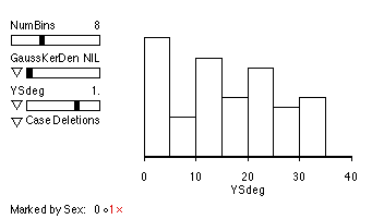
the average years since degree is, you can tell from the scatterplot that
it is much closer to 20 than to 10. Hence the (x - xbar) term that appears
in the SE will be closer to zero if x is 20.
5. What should we do to check the assumptions of the regression model we have applied?
To check that the errors are normally distributed, we could make a normal probability plot of the residuals and verify that the points fall more or less on a straight line. A plot of the residuals vs. years since degree would detect deviations in linearity and also help us catch whether the variance changed as x changed. Note that the p-value and R-squared do NOT help you check any assumptions. In fact, these numbers are really only interpretable if the assumptions hold. Otherwise, they might be deceptive. It is difficult with these data to determine whether the independence assumption is true. Also note that the model does NOT assume that years since degree is normally distributed. And so it does not make sense to make normal probability plots of this.
Incidentally, it makes sense that the variance of the errors would increase as years since degree increases. When people are hired right after their degree, there is probably very little room for negotiation, and so salaries around x=0 should be more or less the same (because the people all look more or less alike.) However, as time goes on and people distinguish themselves in different ways, they might be compensated in a variety of fashions, and so you might start to see more and more disparity as time goes on. This is evident in these data. You can see that the range of salaries for those with less than 5 years since their degree is about$500, while for those with about 30 years since their degree the spread is closer to $1500.
This spread is very apparent in the residual plot of residuals
against YSdeg.
6. An administrator from this college argues that the college doesn't look at the gender of their faculty when making salary decisions. But they do pay attention to how long it has been since the faculty member got his or her degree, and it just so happens at their university, on average their female faculty are younger than their male faculty. That is why there is a perceived disparity. What do you think of this argument, in light of the data here in section B? (Don't try any statistical tests. Just look at the data.) Do the data in B contradict what you concluded in part A? Explain.
Of course whether or not you see a contradiction
depends on your answer to part A. The basic idea behind this question is
as follows: We know that salary varies a great deal among the faculty,
and part A suggests there is some evidence that part of this variation
is because of gender. (Or perhaps you concluded the opposite.) The regression
analysis in part B fairly convincingly demonstrates that years since degree
plays a big role in salary assignments, but it doesn't account for all
(or even most) of the variation among faculty members. So the administrator's
argument is not very strong. It does not eliminate the possibility that
gender still plays a role. Interestingly, if you look at the regression
line, you'll find that only 3 of the fourteen women have salaries above
the regression line. If there were no differences in gender, we would expect
about half of the women to be above and half below. (If you want, you can
calculate the probability, under this assumption, of having 3 or fewer
women above the line -- use a binomial distribution with p = .5, n = 14.)
This means that 11 of 14 women make less than the average amount of those
with the same number of years since their degree. This suggests that there
might be some bias.
If you want to follow up on your own, the data are available
at http://www.stat.ucla.edu/~rgould/110as99/datalist.html.
You might want to look to see what happens to these analyses
and our conclusions if you remove the outlier -- the one woman who made
more than anyone else.
END OF QUESTIONS -- ARC OUTPUT FOLLOWS
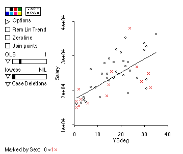
2. Here's the output from a regression.
Data set = Pay, Name of Fit = L2
Normal Regression
Kernel mean function = Identity
Response = Salary
Terms = (YSdeg)
Coefficient Estimates
Label Estimate Std. Error t-value
Constant 17502.3 1149.70 15.223
YSdeg 390.645 60.4109 6.466
R Squared: 0.455428
Sigma hat: 4410.12
Number of cases: 52
Degrees of freedom: 50
Summary Analysis of Variance Table
Source df SS MS F p-value
Regression 1 813271618. 813271618. 41.82 0.0000
Residual 50 972458240. 19449165.