Below is a list of some of the projects I have worked on. Note that this page utilizes MathJax rendering of LaTeX code.
Classification algorithms are some of the most important machine learning techniques available today. As a supervised learning method, the scientist is given a dataset \( D = \{ (x_i, y_i) : i\leq m\} \), with feature vectors \( x_i \in \mathbb{R}^d \) and class labels \( y_i\). The goal for the scientist is to construct a function \( f(x) \) that can classify a vector of features \(x \) to its class \(y\) with high accuracy.
Adaboost is a classification algorithm in machine learning that utilizes a family \( \Delta = \{ h_t (x)\} \) of weak classifiers to build a stronger classifier \(H(x) \); in practice, \( |\Delta| \) is on the order of \(10^3\) to \(10^5\). In the two-class case (such as "is a face" or "is not a face" for images), the weak classifiers \( \{ h_t(x) \} \) need only have error rates strictly less than 50%. The strong classifier \(H\) is a linear combination of the weak classifiers Adaboost algorithm builds the strong classifier \(H\) as a linear combination of weak classifiers in \( \Delta \), sequentially picking the weights \( \alpha_t \) that are the coordinates of \(H \) in terms of the \( \{ h_t \} \). Adaboost does this by carefully constructing weights for each datum \( (x_i, y_i)\) and sequentially choosing the least (weighted) error classifier at each stage of the algorithm, then updating the weights of the data iteratively so that data that are incorrectly classified receive more attention in the next round of the selection process. The process terminates when a desired accuracy is reached, or when the number of terms in the expansion for \( H\) is large enough (on the order of \( 10^2 \) to \(10^3 \) terms, usually).
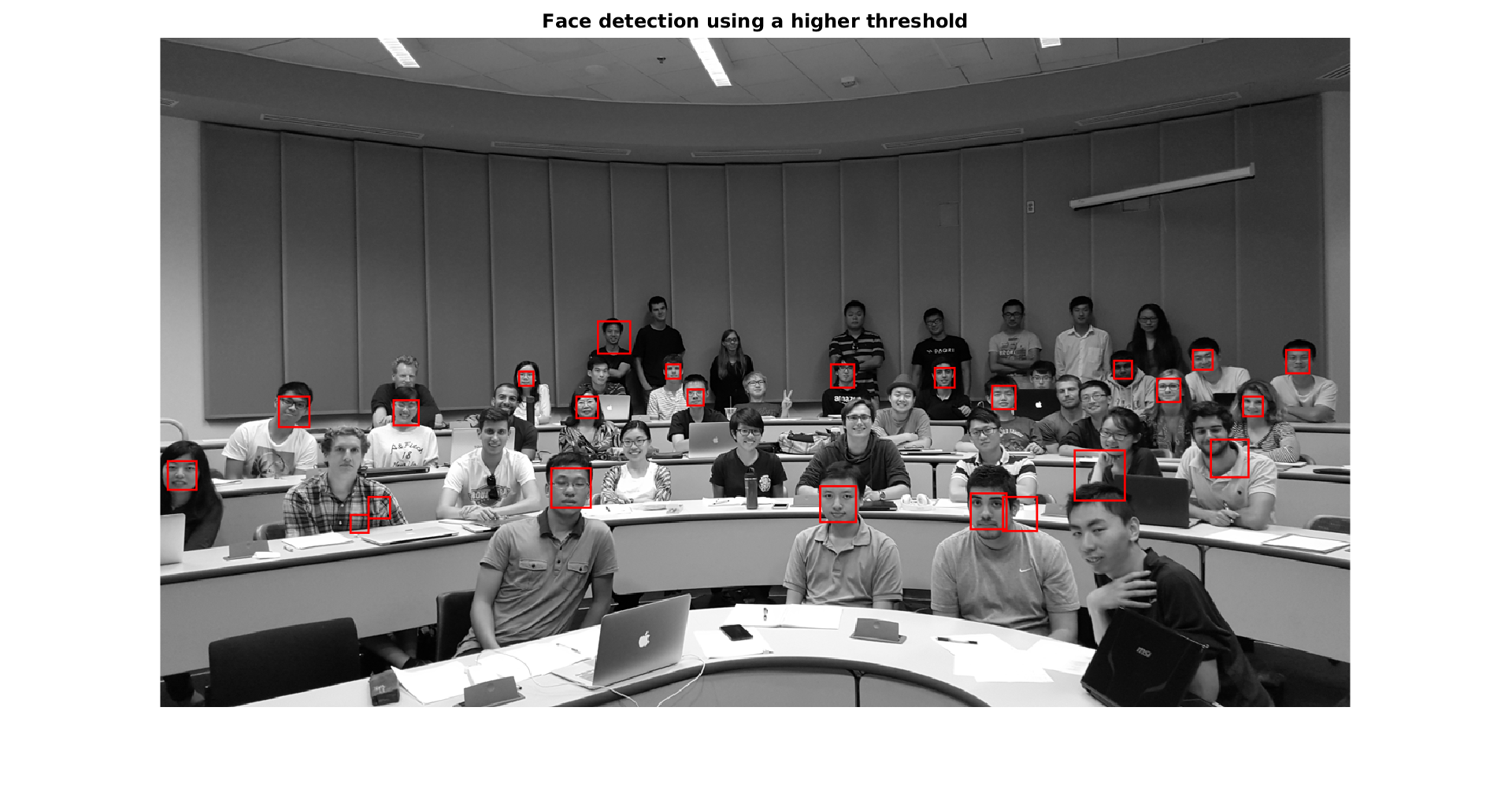
For a class project, I worked on using Adaboost to detect faces on images. I constructed a family of \( \approx 10^4 \) weak classifiers \( \Delta \) using Haar features on a training set of images that consist of \( \approx 10^3 \) faces and non-face images alike that appear on \( 16\times 16\) pixel grids. The resulting strong classifier was nearly 100% accurate on the testing images (using k-fold validation). Of course, we are interested in seeing if this algorithm will accurately find faces in any picture, not just \( 16\times 16\) pixel windows like in the training data. This problem is slightly nontrivial because there may be multiple faces of different sizes and orientations, which may preclude our classifier from immediately working effectively. A crude way of getting around this is to test all squares of different sizes in the testing image, resize the square subimages to be \( 16\times 16 \), then run the classifier on these. The resulting 'found faces' will then have many overlaps, and then of those squares that overlap in a particular area, we choose the square with the highest 'face score' as the 'real face'. The results of doing this may be found here.
One can construct a discrete-time mathematical SIR (susceptible, infected, recovered) epidemic on a graph \(G = (V,E)\) by partitioning the elements in \(V\) into one of three sites: susceptible \((x\in \xi_n)\), infected \((x\in \eta_n)\), and recovered \((x\in \rho_n)\). We start from an initial configuration of susceptible and infected sites (say, \(\eta_0 = \{ 0\}\), \(\xi_0 = V \setminus \eta_0\), and \(\rho_0=\emptyset\)), and we consider a fixed parameter \(p\in (0,1)\) that is the probability that any infected site \(x\in \eta_n\) infects a neighboring susceptible site \(y\in \xi_n\) (so that \((x,y)\in E)\). Infected sites remain infected for one unit of time, and then become `recovered’, and may no longer infect any other sites (or become infected again); that is, \(x\in \eta_n\) means \(x\in \rho_{n+1}\). We then let the process run for times \(n=1, 2, \dots\) and examine the behavior of the infected sites \(\eta_n\).
There are two possible behaviors for the epidemic: either the epidemic dies out in finite time almost surely (i.e., \(\eta_n = \emptyset\) eventually), or with positive probability the epidemic continues forever, so that at any given time \(m\), there is at least one site \(x\in \eta_m\). In the latter case, we say that infection occurs in the epidemic. Since each edge \((x,y)\) in the epidemic process is `used’ precisely once—when either \(x\) attempts to infect \(y\) or vice-versa—there is a correspondence between infections occurring in a graph \(G\) and percolation occurring in the same graph: an infection occurs in \(G\) iff percolation occurs in \(G\). Standard percolation theory shows that there exists a critical value \(p_c(G)\) for the probability \(p\) such that when \(p>p_c\), infection occurs, and for \(p<p_c\), the epidemic dies out almost surely.
I studied this process on the graph \(\mathbb Z^d\), with an edge set \(E = E_R\) parameterized by a quantity \(R\), such that there are edges between two sites \(x,y\in \mathbb Z^d\) iff \(|x-y|_{\infty} \leq R\), where \(|\cdot|_\infty\) denotes distance in the \(\ell^\infty\) metric. As the graph is parameterized by \(R\), the corresponding critical value \(p_c\) is likewise paramaterized by \(R\). In my masters thesis, I proved a lower bound on the critical value for percolation, as a function of \(R\), in dimensions \(d=2\) and \(d=3\) by studying the corresponding SIR epidemic. A paper on this result is currently in preparation with Ed Perkins.
 Geothermal heat pump
systems (also known as ground-source heat pump systems, or GSHP) are an
incredibly energy-efficient way to heat and cool a home. Traditional heat pumps rely on a heat
exchanger that exchanges heat with air, which functions as a heat
source/sink. Geothermal heat pump systems utilize the fact that just a
few meters below the surface, the ground is nearly constant temperature
year-round, and hence use the soil as a heat source/sink. The heat
exchanger takes the form of a liquid running through pipes that are burrowed
underground. As the temperature of the soil is near-constant year
round, the heat pump is also able to function effectively year-round, as the
liquid through the pipes deposits heat into the soil in the summer, and
receives energy from the soil in the winter. The pipes may be situated in a
number of networks, most of which are described at the Department
of Energy website.
Geothermal heat pump
systems (also known as ground-source heat pump systems, or GSHP) are an
incredibly energy-efficient way to heat and cool a home. Traditional heat pumps rely on a heat
exchanger that exchanges heat with air, which functions as a heat
source/sink. Geothermal heat pump systems utilize the fact that just a
few meters below the surface, the ground is nearly constant temperature
year-round, and hence use the soil as a heat source/sink. The heat
exchanger takes the form of a liquid running through pipes that are burrowed
underground. As the temperature of the soil is near-constant year
round, the heat pump is also able to function effectively year-round, as the
liquid through the pipes deposits heat into the soil in the summer, and
receives energy from the soil in the winter. The pipes may be situated in a
number of networks, most of which are described at the Department
of Energy website. 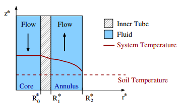 I worked with Burt Tilley, Kathryn
Lockwood, Greg Stewart, and Justin Boyer to develop a mathematical model of
the heat exchange occurring between the water in the pipes, the pipe walls,
and the soil in a specific piping system known as the concentric vertical
pipe. In this pipe, water flows down from the home through an inner
cylindrical cavity, and flows back up the pipe to the home through an outer
cylindrical cavity. The diagram to the left depicts the system in
action during summer, as the water decreases in temperature as it exchanges
heat from the soil. The pipes are designed so that the inner pipe
material in the region \(R_0^* < r^* < R_1^*\) has low conductivity
while the outer pipe material at \(r^* = R_2^*\) is highly conductive.
Our model studied the heat exchange as a function of design parameters such
as the spacing of the inner and outer pipes, the flow rate, and the length
of the pipe. We developed a characteristic length at which heat
exchange occurs in the soil, and found that one could drill less deeply
while still retaining the vast majority of heat exchange ability of the
system. These results
were published in the Journal of Engineering Mathematics in 2014.
I worked with Burt Tilley, Kathryn
Lockwood, Greg Stewart, and Justin Boyer to develop a mathematical model of
the heat exchange occurring between the water in the pipes, the pipe walls,
and the soil in a specific piping system known as the concentric vertical
pipe. In this pipe, water flows down from the home through an inner
cylindrical cavity, and flows back up the pipe to the home through an outer
cylindrical cavity. The diagram to the left depicts the system in
action during summer, as the water decreases in temperature as it exchanges
heat from the soil. The pipes are designed so that the inner pipe
material in the region \(R_0^* < r^* < R_1^*\) has low conductivity
while the outer pipe material at \(r^* = R_2^*\) is highly conductive.
Our model studied the heat exchange as a function of design parameters such
as the spacing of the inner and outer pipes, the flow rate, and the length
of the pipe. We developed a characteristic length at which heat
exchange occurs in the soil, and found that one could drill less deeply
while still retaining the vast majority of heat exchange ability of the
system. These results
were published in the Journal of Engineering Mathematics in 2014.