Unsupervised Learning of Compositional Sparse Code for Natural Image Representation
Hong Yi, Zhangzhang Si, Wenze Hu, Song-Chun Zhu, and Ying Nian Wu
Report |
Talk |
Latex
This article proposes an unsupervised method for learning compositional sparse code for representing natural images.
Our method is built upon the original sparse coding framework where there is a dictionary of basis functions often
in the form of localized, elongated and oriented wavelets, so that each image can be represented by a linear combination
of a small number of basis functions automatically selected from the dictionary. In our compositional sparse code, the
representational units are composite: they are compositional patterns formed by the basis functions. These compositional
patterns can be considered shape templates. We propose an unsupervised learning method for learning a dictionary of
frequently occurring templates from training images, so that each training image can be represented by a small number
of templates automatically selected from the learned dictionary. The compositional sparse code translates the raw image
of a large number of pixel intensities into a small number of templates, thus facilitating the signal to symbol transition
and allowing a symbolic description of the image. Experiments show that our method is capable of learning meaningful
compositional sparse code, and the learned templates are useful for image classification.
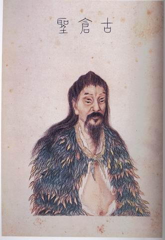
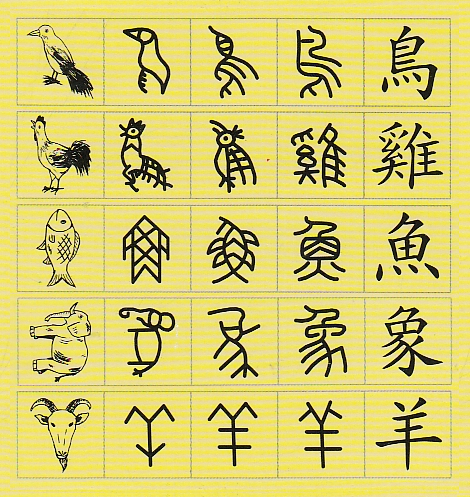
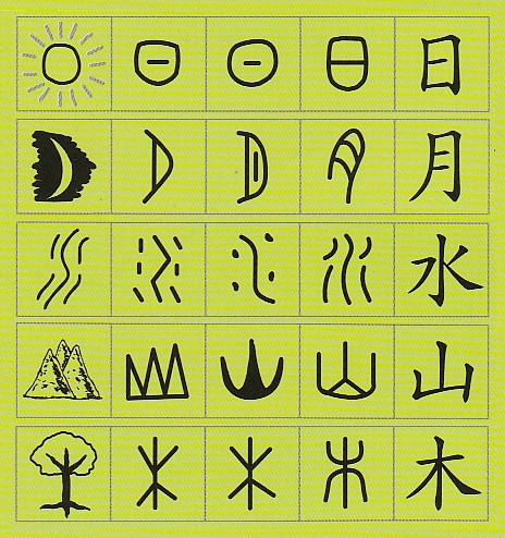
As illustrated by the above figure, the ancient Chinese (or a mythology figure with four eyes) developed the early form of Chinese characters as a coding scheme
for representing natural images where each character is a pictorial description of a pattern. The early pictorial form then
gradually evolved into the form that is in use today. The system of Chinese characters can be considered a compositional
sparse code: each natural image can be described by a small number of characters selected from the dictionary, and each
character is a composition of a small number of strokes. The goal of this paper is to develop a compositional sparse code
for natural images. Our coding scheme can be viewed as a mathematical realization of the system of the Chinese characters.
In our compositional sparse code, each ``stroke'' is a linear basis function such as a Gabor wavelet, and each ``character''
is a compositional pattern or a shape template formed by a small number of basis functions.
(a)  (b)
(b) 
 (c)
(c) 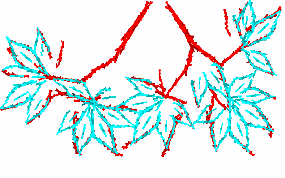 (d)
(d) 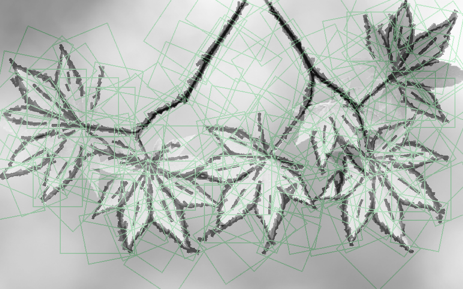 (e)
(e) 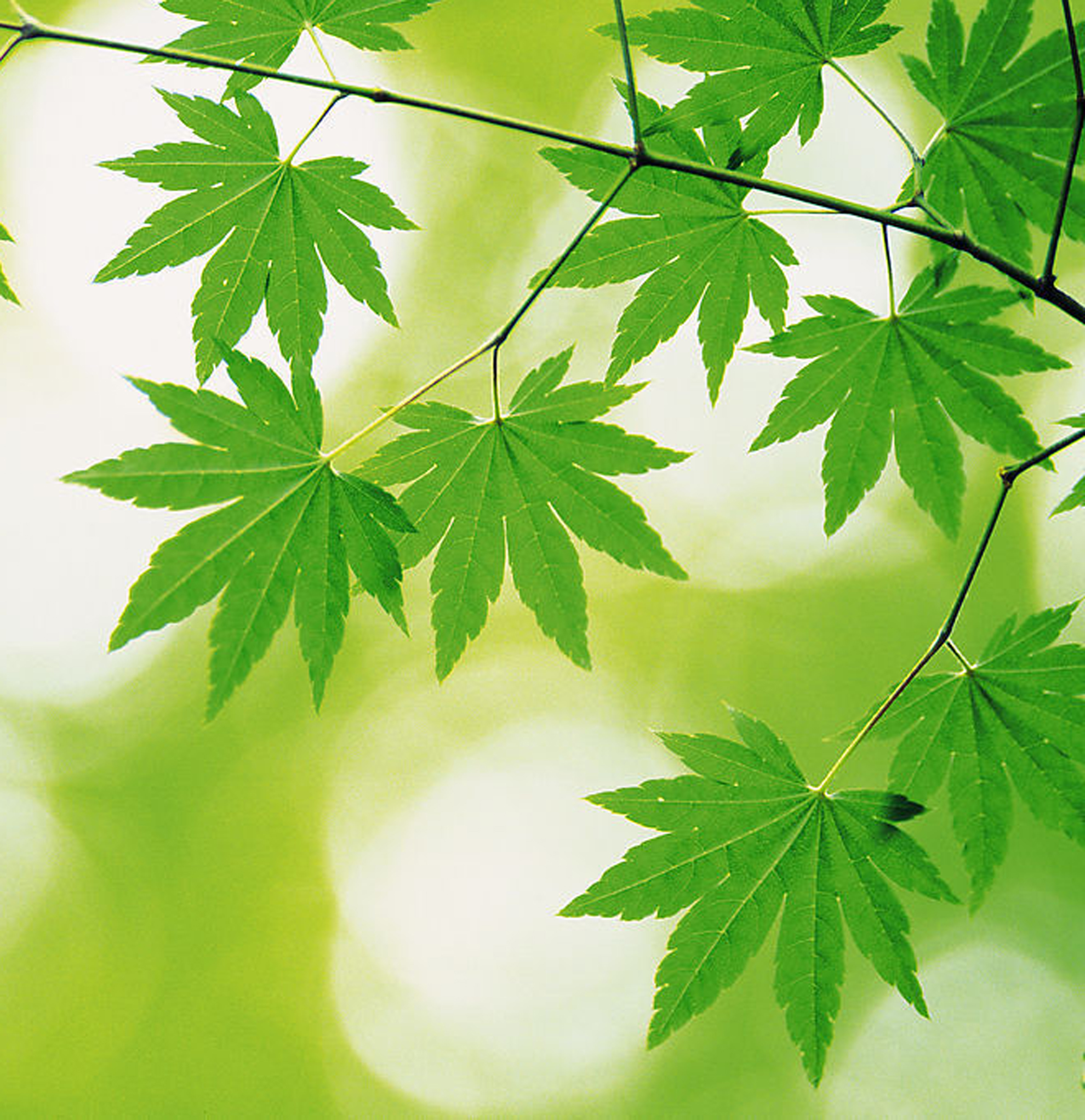 (f)
(f) 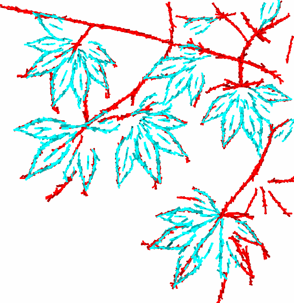
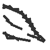
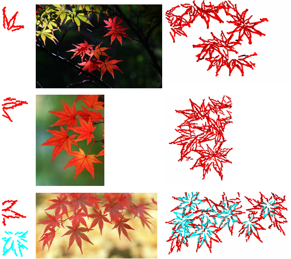
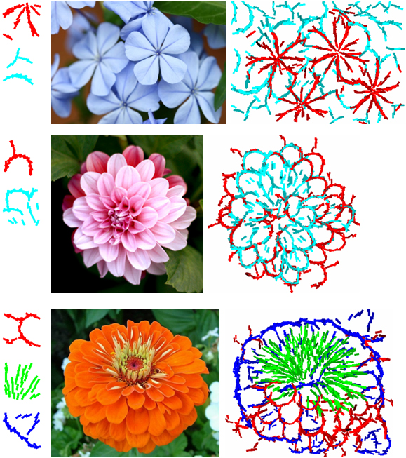
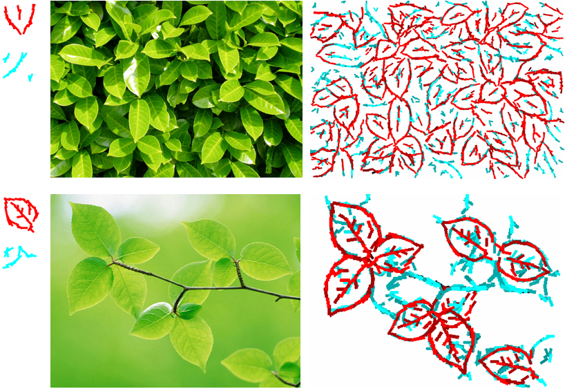
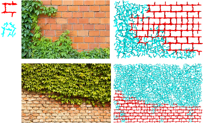
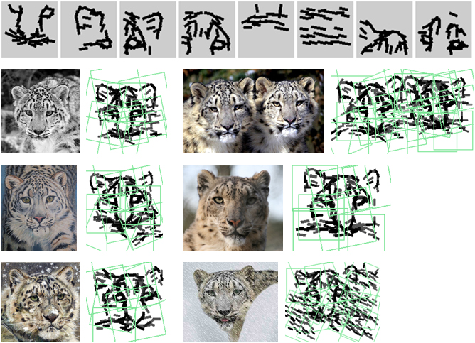
(a) Training image of 480 by 768 pixels. (b) 2 compositional patterns of Gabor wavelets in the form of
active basis templates learned from the training image. Each Gabor wavelet is illustrated by a bar with the
same location, orientation and length as that wavelet. The bounding box of the templates is 100 by 100 pixels.
The numbers of Gabor wavelets are respectively 22 in the red pattern and 40 in the green pattern. The number
of templates and the number of wavelet elements in each template are automatically determined.
(c) Representing the training image by translated, rotated, scaled and deformed versions of the 2 templates.
(d) Superpose deformed templates on the original image. Green squared boxes are bounding boxes of the templates.
(e) Testing image. (f) Representation of the testing image by the 2 templates.
The unsupervised learning algorithm starts from templates learned from randomly cropped image patches,
so the initial templates are rather random. The algorithm then iterates the following two steps: (1) Encoding each
training image by translated, rotated, scaled and deformed versions of the current vocabulary of templates,
by a template pursuit process. (2) Re-learning each template from image patches currently encoded by this template,
by a shared pursuit process.
(a) 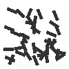


 (b)
(b) 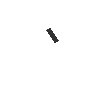
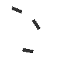
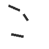
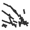
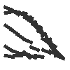
(a) Template of leaf learned in the first 7 iterations of the unsupervised learning algorithm.
(b) In each iteration, the shared pursuit process selects wavelet elements sequentially to form
the template. The sequence shows the process selecting 1, 3, 5, 10, 20, 30, 40 wavelet elements
in the last (10th) iteration.
More results:
Data and code for experiments on image representation
The following are the links to the code and data of some experiments on image representation. For each set of experiments,
the one marked with full name (e.g., "Maple 2") is the one that achieves the maximum BIC.
To reproduce the results shown below, please download "ABC.zip", unzip it and enter the folder "ABC", enter Matlab,
and type "StartFromHere". After the code finishes running, go to the "document" folder, and click "ABC.html".
For exact reproducibility, please always re-start your matlab (our version is Matlab R2009b) before running
"StartFromHere". You can play with the code by changing the parameter setting in ParameterCodeImage.m
The following experiments use the common parameter setting (these parameters are not that essential): The size
of each active basis template is 100 (width) by 100 (height) pixels. The maximum number of Gabor elements in each template
is 40, and the actual number of automatically determined. For Gabor wavelets we use a scale of 0.70 and 16 quantized
orientations. Each Gabor element is allowed to move 3 pixels along its normal direction and rotate 1 orientation step
at most. The saturation level is 6 after local normalization within a neighborhood of 20 by 20 pixels. In the encoding step,
the activated templates need to have a SUM2 score of at least numElement times gamma, where gamma = 1. For local inhibition
between templates, a template with a squared bounding box of side length D inhibits a circular area of radius rho times D
from its center, so that no other templates are allowed to center within the inhbited area. rho = .4.
1 |
Maple 2 |
3 |
4 |
Low resolution ---
1 |
2 |
Maple Large 3 |
4 ---
1 |
2 |
Maple Small 3 |
4 ||
another example ||
another example ||
another example ||
another example ||
another example ||
another example ||
another example ||
another example ||
another example ||
another example ||
another example ||
another example
1 |
Leaf 2 |
3 |
4 ||
another example ||
another example ||
another example ||
another example ||
another example ||
another example ||
another example ||
another example ||
another example ||
another example
1 |
Leaf 2 |
3 |
4 ||
another example
1 |
Ivy 2 |
3 |
4 ||
another example ||
another example
1 |
Lotus 2 |
3 |
4 |
Low resolution ||
another example
1 |
Daisy 2 |
3 |
4 ||
another example ||
another example
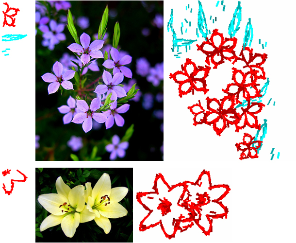
1 |
Flower 2 |
3 |
4 ||
another example ||
another example ||
another example ||
another example ||
another example ||
another example ||
another example ||
another example ||
another example
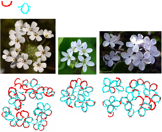
1 |
Flowers 2 |
3 |
4 ||
another example ||
another example ||
another example ||
another example ||
another example ||
another example ||
another example ||
another example
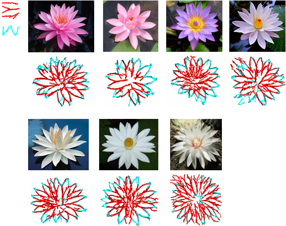
1 |
2 |
Waterlily 3 |
4 ||
another example ||
another example ||
another example ||
another example ||
another example ||
another example ||
another example
1 |
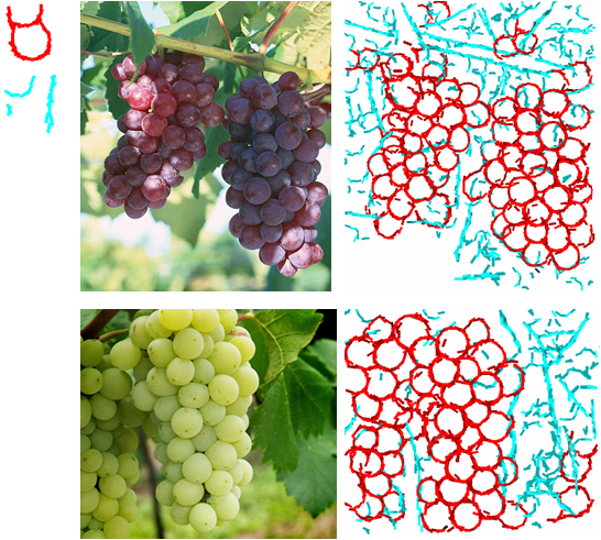
Grape 2 |
3 |
4 ||
another example
1 |
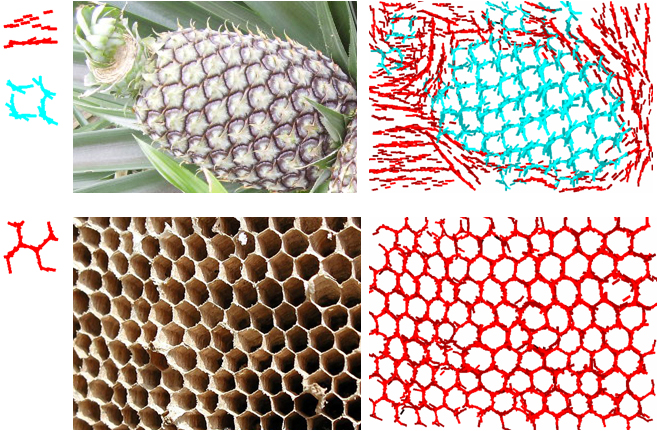
Pineapple 2 |
3 |
4 |
Low resolution
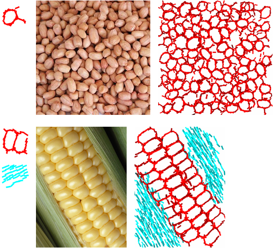
Peanut 1 |
2 |
3 |
4
1 |
Corn 2 |
3 |
4 |
Low resolution
Beehive 1 |
2 |
3 |
4 ||
Another example
1 |
Brick ivy 2 |
3 |
4
Brickwall 1 |
2 |
3 |
4 |
Low resolution ||
another example ||
another example ||
another example ||
another example (multiscale)
1 |
Stone wall 2 |
3 |
4 |
Low resolution
1 |
2 |
Pavement 3 |
4 ||
another example
1 |
2 |
3 |
Brick pavement 4 |
5 ||
another example
1 |
Pebble 2 |
3 |
4 ||
another example
1 |
Net 2 |
3 |
4 ||
another example ||
another example ||
another example ||
another example ||
another example ||
another example ||
another example
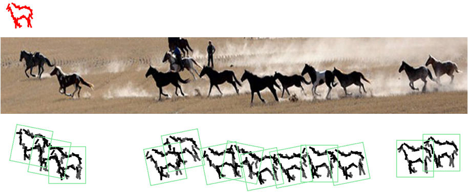
Horse 1 |
2 |
3 |
4 ||
another example ||
another example
2 |
4 |
6 |
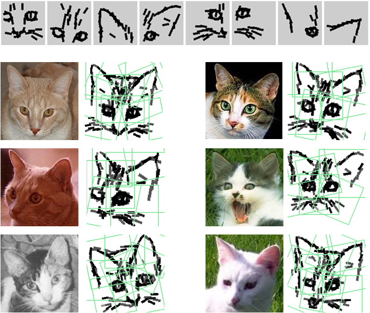
Cats 8 |
10 |
12
Snow leopard
10 |
20 |
Animal 30
10 |
Cuppot 20 |
30
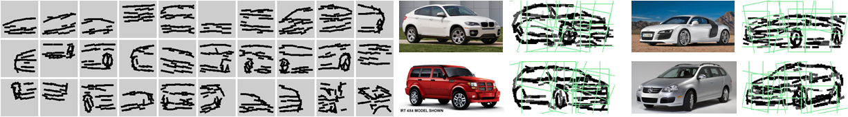
10 |
20 |
Car 30
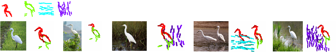
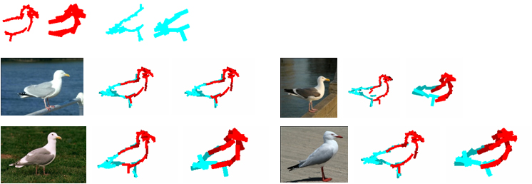
Egret
Bird
Swan
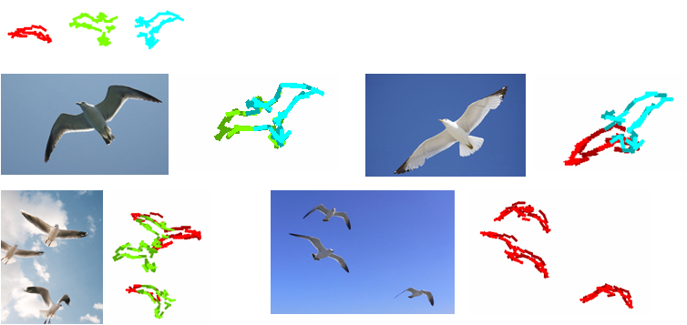
Seagull (multi-scale)
Seagull flying
Cougar
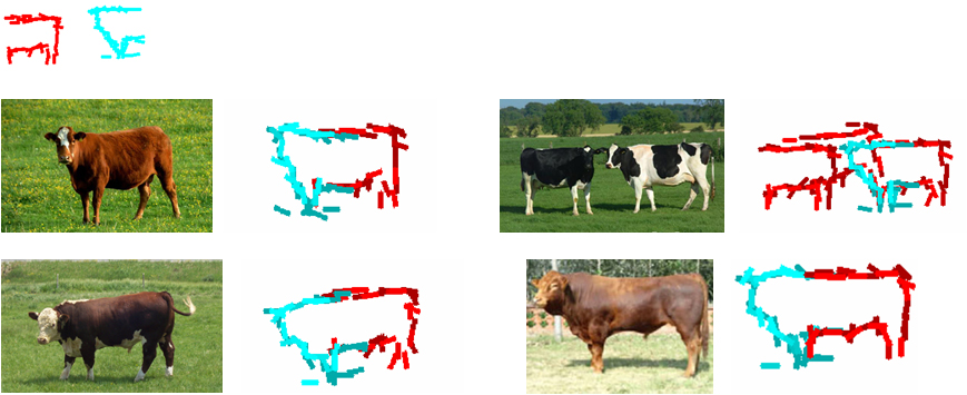
Cattle
Data and code for experiments on image classification
The learned vocabulary of active basis models (size = 100 by 100, number of wavelet elements = 30) can be used as
feature extractors for image classification. For each image (resized to 150^2 while keeping aspect ratio), we scan
each active basis template over this image, at 3 resolutions and orientations. For each of the 3 orientations, we
then take the maximum score of the log-likelihood over the whole image and over all the three resolutions. The number
of templates is T = 10, so this gives us 3T scores for each image. We feed these 3T dimensional feature vector to a
linear logistic regression regularized by l-2 norm. We compare the performance of this simple classifier with SVM
based on SIFT with 50, 100, 500 codeworks obtained by k-means clustering, either with linear SVM or SVM based on
histogram intersection kernel. We take the best of these 6 results and compare it with our method. All experiments
are carried out with 5 independent runs and the 95 percents confident intervals on accuracies are calculated. The
following are the results. Please click the links in the table for data and code.
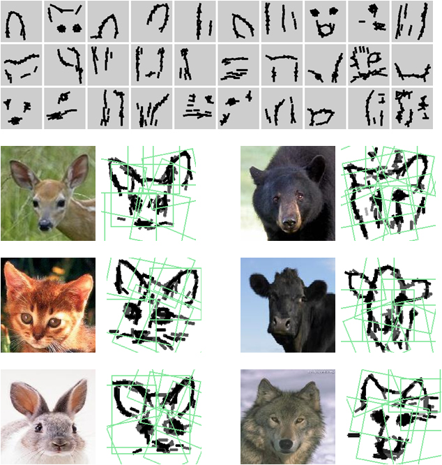
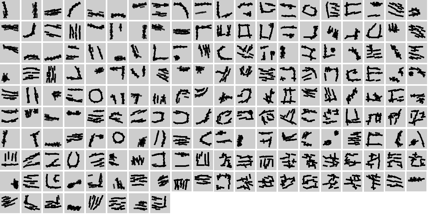
We also test our method on the whole Caltech-101 data set with the following modifications:
(1) We learn T=200 templates from all 101 categories together. Each template is of the size 64 by 64 with 15 wavelet elements.
The following figure displays these templates (some templates disappear because they fail to encode enough number of image patches).
(2) For each image, and for each template at each orientation, besides the global maximum, we also divide the image
equally into 2 by 2 sub-regions and take the maximum within each sub-region. In addition to each maximum, we
also take the corresponding average. So each template extracts 30 features from the image. Thus in total,
each image produces a 30T-dimensional feature vector.
We adopt standard evaluation protocol. For 15 training images per category, the accuracy of our method is 61.6 ± 2.2.
For 30 training images per category, our result is 68.5 ± 0.9. While more recent papers report better performances
based on spatial pyramid matching, we do not use k-means to further cluster response maps into another layer of codewords,
neither do we use any kernel.
Code on Caltech 101