Note: Below were experiments done at the early stage of this project.
See THIS PAGE for more recent experiments where local shift leads to cleaner templates.
Parameters
In the experiments in this article, we hand pick the number of basis elements, $n$.
In principle, it can be automatically determined by comparing $\sum_{m=1}^{M}
h(r_{m, i})/M$ with the average of $h(\M1_m(x, y, s, \alpha))$ in natural images or
in the observed image $\I_m$. If the former is no much greater than the latter, we
should stop the algorithm. We also hand pick the resize factor of the training
images. Of course, in each experiment, the same resize factor is applied to all
the training images.
Parameter values. The following are the parameter values that we used in all the
experiments in the IJCV paper (unless otherwise stated). Size of Gabor wavelets =
$17 \times 17$ (scale parameter = .7). We have extended the code so that we can learn templates using
Gabors at multiple scales. $(x, y)$ is sub-sampled every 2 pixels. The orientation
$\alpha$ takes $A = 15$ equally spaced angles in $[0, \pi]$. The orthogonality
tolerance is $\epsilon = .1$. The threshold is $T = 16$ in the threshold
transformation. The saturation level $\xi = 6$ in the sigmoid transformation.
The shift along the normal direction $d_{m, i} \in [-b_1, b_1] = [-6, 6]$ pixels.
In later experiments, we sometimes reduce it to 4 or 3, and we use local normalization
of filter responses.
The shift of orientation $\delta_{m, i} \in [-b_2, b_2] = \{-1, 0, 1\}\times \pi/15$.
Experiments 1 and 2
Supervised learning and detection
In experiment 1, we learn the template from images with given bounding boxes.
In experiment 2, we use the learned template to detect and sketch the object.
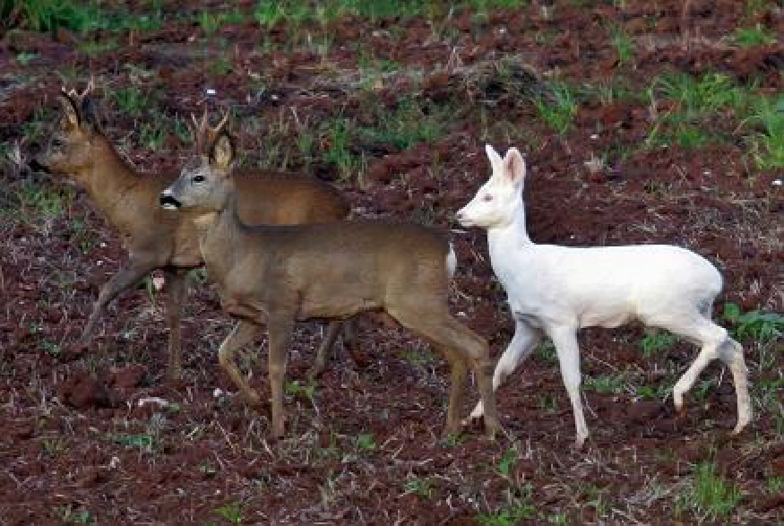
Negative experience in Experiment 1. This experiment requires that the training
images are roughly aligned and the objects are in the same pose. If this is not
the case, our method cannot learn clean templates. In later experiments, we
show that our method can be extended so that we can learn from non-aligned images
and find clusters in training images.
Also, our method does not do well on objects with strong textures, such as zebras,
leopards, tigers, giraffes, etc. The learning algorithm tends to sketch edges in
textures. This suggests that we need stronger texture model, as we discussed
in the subsection about adaptive texture background.
Negative experience in Experiment 2. Our method can sometimes be distracted
by cluttered edges in the background. We need to combine templates at multiple
resolutions to overcome this problem. This has already been implemented, but
has not been thoroughly tested. We also need to include flatness and texture
variables in the model. Again this has been done but has not been tested.
(a) Prototype code
The above code is simple and convenient for development purpose. But it is not
optimized for speed.
(a.1) matching pursuit
Earlier code for matching pursuit. Linear additive representation and matching
pursuit are the prototype machinery for the present work.
(a.2) Edge detection
Earlier code for edge detection based on non-maximum suppression. Multi-scale Gabor filters are used.
(0) Code and data
==> Number of training images = 9; Number of elements = 50; Length of Gabor = 17 pixels; Local normalization or not = 1; Range of displacement = 6 pixels; Subsample rate = 1 pixel; Image height and width = 122 by 120 pixels

==> Number of testing images = 101; The search is over 10 resolutions,
from 10% to 100% of the testing image.


(1)
Our first experiment based on old code (2007) data source: yahoo auto page
(1.1) code
with whitening (2007)
(1.2) code
with sigmoid transformation (2007)
(1.3)
Code with sigmoid transformation and normalization within scanning window (May 2009)
The sigmoid model proves to be more accurate according to the classification experiments.
Normalizing filter responses within scanning window produces more reliable likelihood scores
in detection.
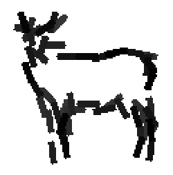
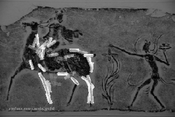
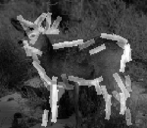
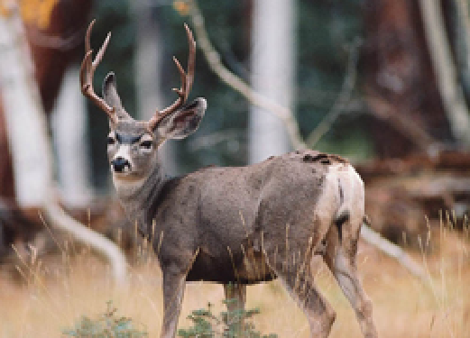
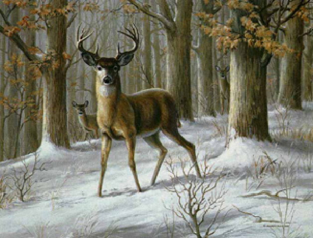
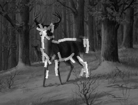
The following result is produced by code in (1).
The 37 training images are 82*164. The first block displays the
learned active basis consisting of 60 elements. Each element is symbolized by a bar.
The rest of the blocks display the observed images and the corresponding deformed
active bases. The images are displayed in the descending order of the log-likelihood
ratio, which scores the template matching.
eps
(1.4) code
with sigmoid transformation, within-window normalization, with q() pooled
from 2 natural images. (June 2009)
 eps
eps
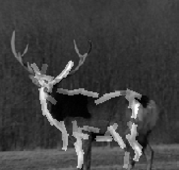
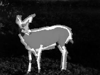
Learned template from training images.

 eps
eps
 eps
eps
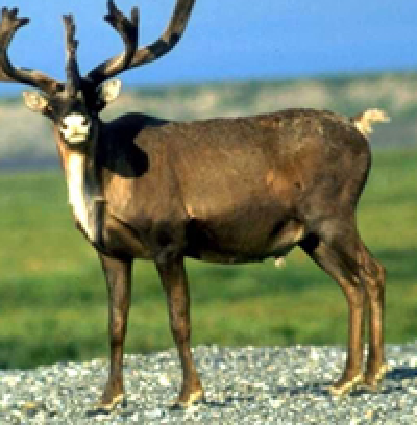
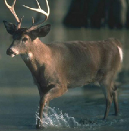
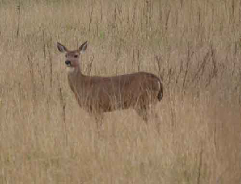
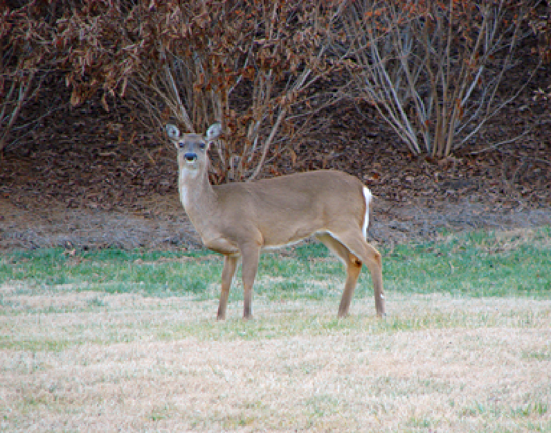
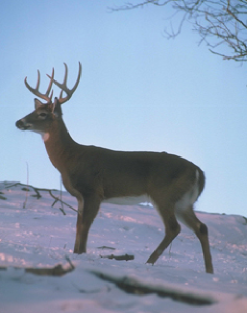
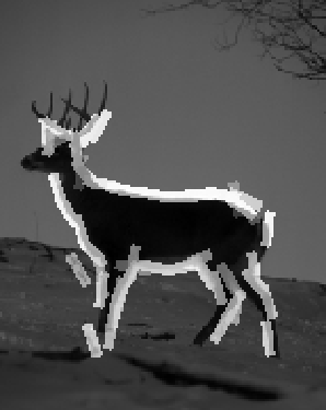
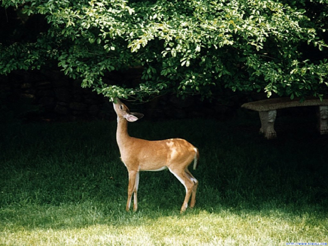
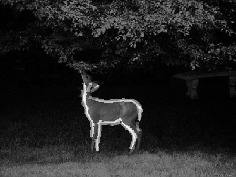
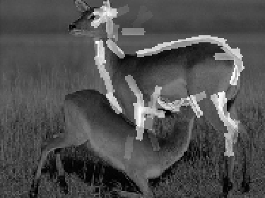
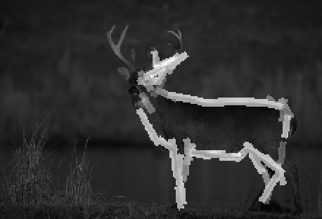
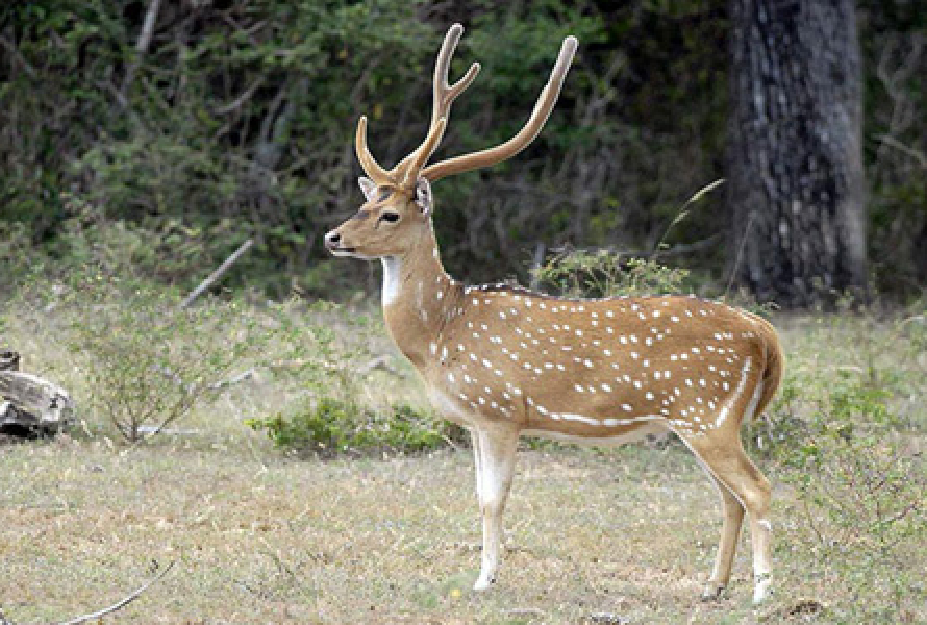
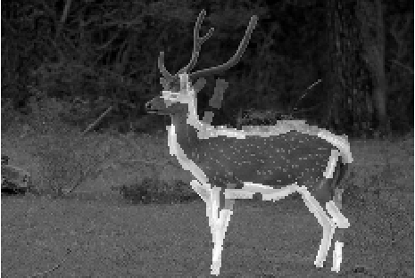
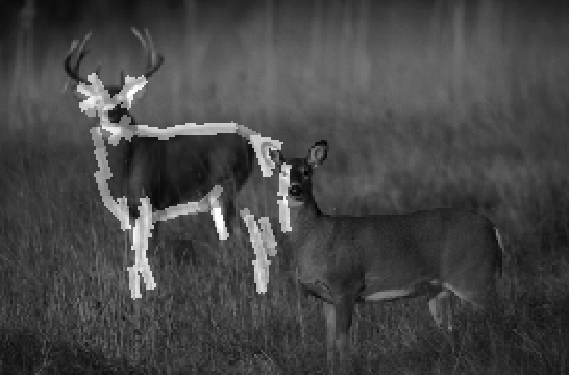
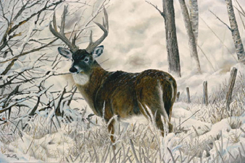
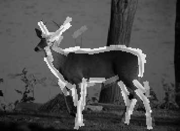
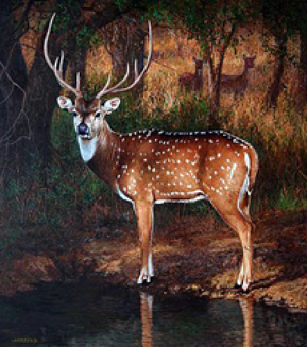
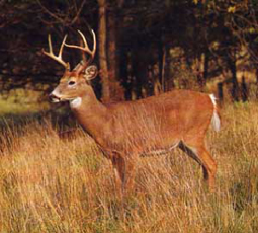
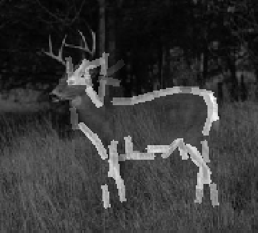
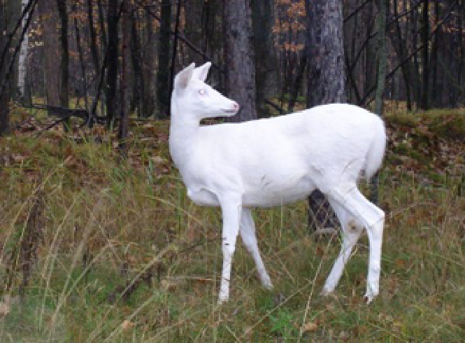
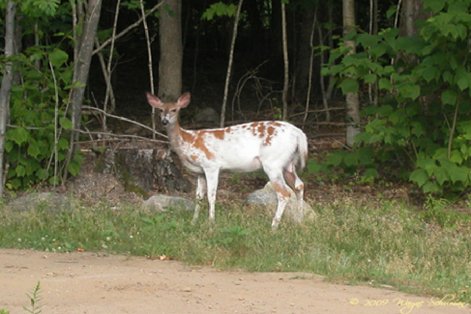
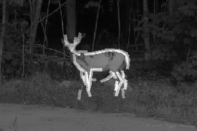
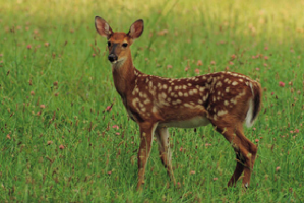
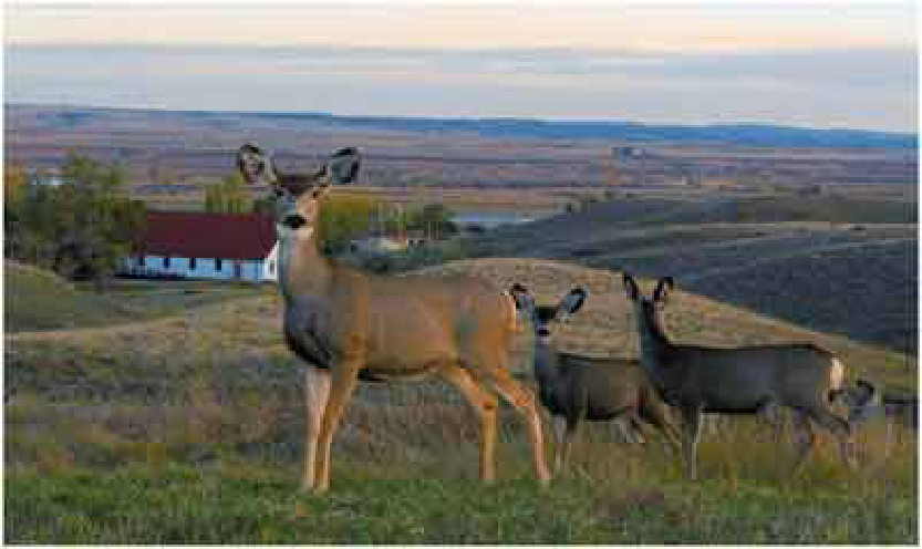
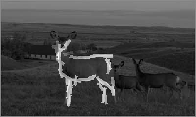
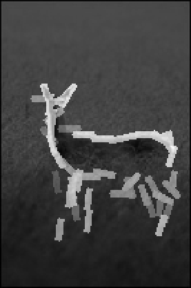
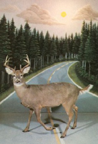
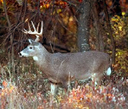
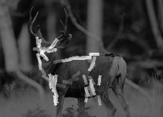
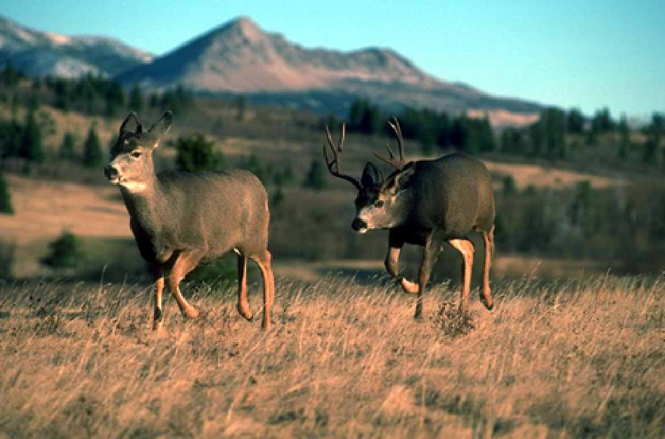
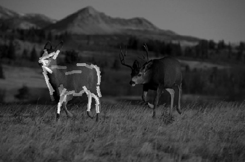
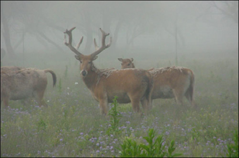
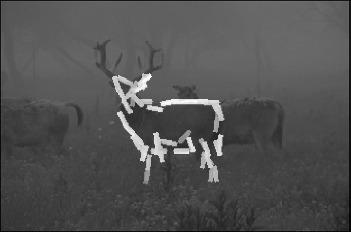
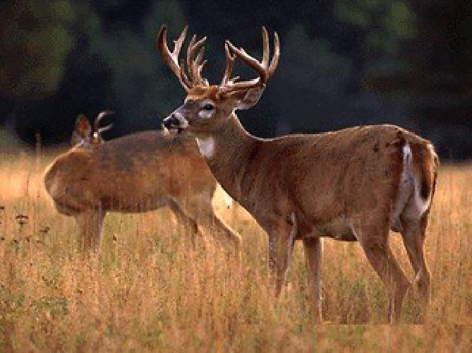
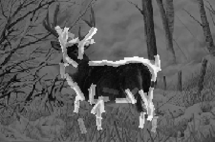
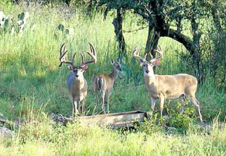
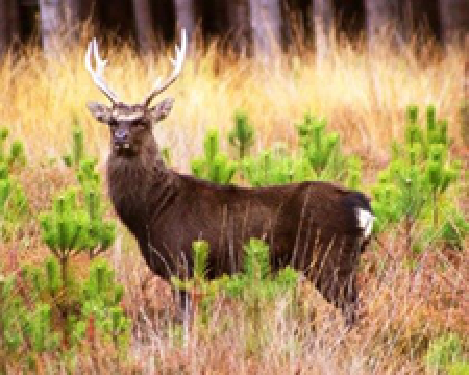
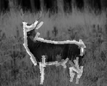
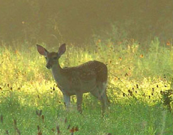
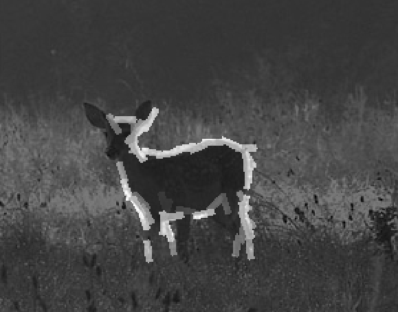
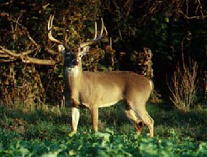
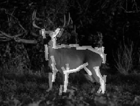
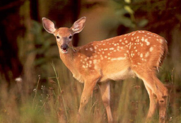
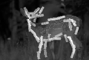
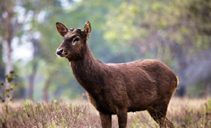
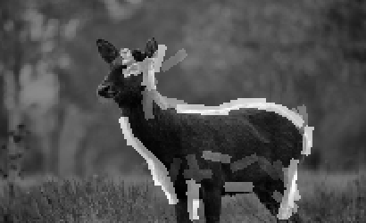
Left: Testing image. The recognition algorithm is run on 15 resolutions,
from 50x67 to 751x1001.
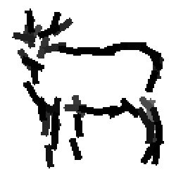
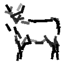
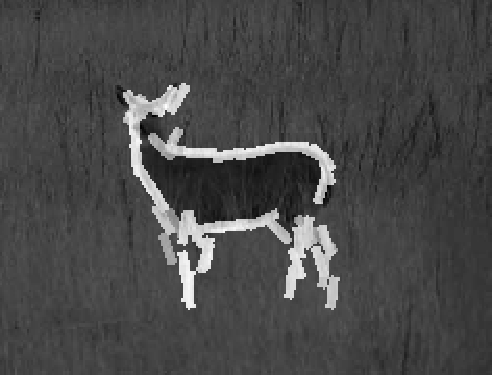
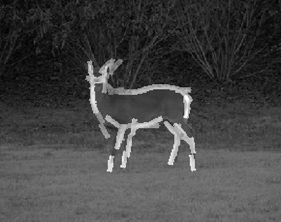
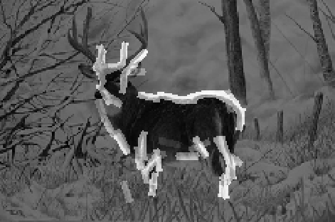
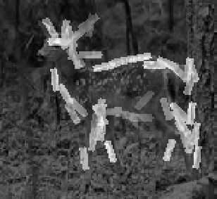
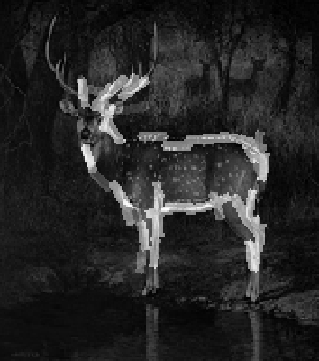
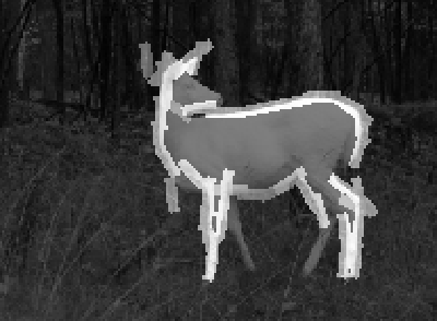
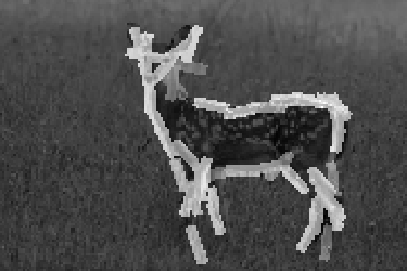
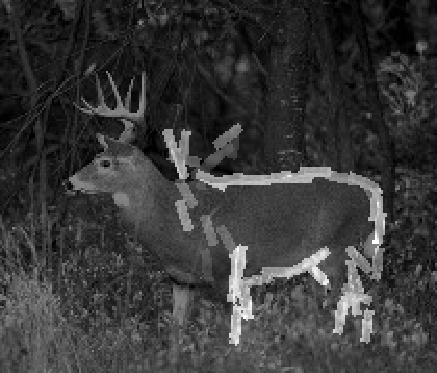
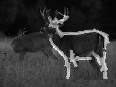
Right: Superposed with sketch of the 60 elements of the deformed active basis at the
optimal resolution.
 eps
eps
 eps
eps
Left: MAX2 scores at resolutions 1 to 15.
Right: SUM2 map at the optimal resolution.
(1.5) code
with local normalization (August 2009)
(1.6)
code with plotting sum-max maps (2008)
(2)
Code with sigmoid transformation and normalization within scanning window.
(May 2009) data source: internet
(2.1) code
with sigmoid transformation, within-window normalization, with q() pooled
from 2 natural images. (June 2009)
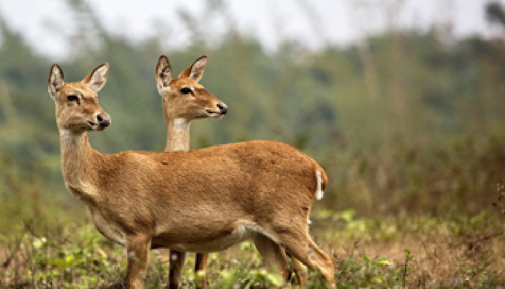
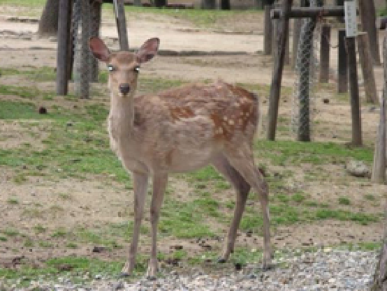
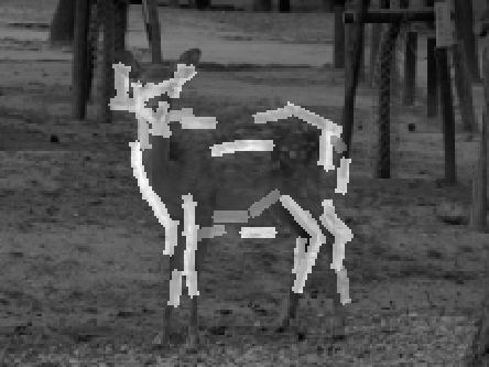
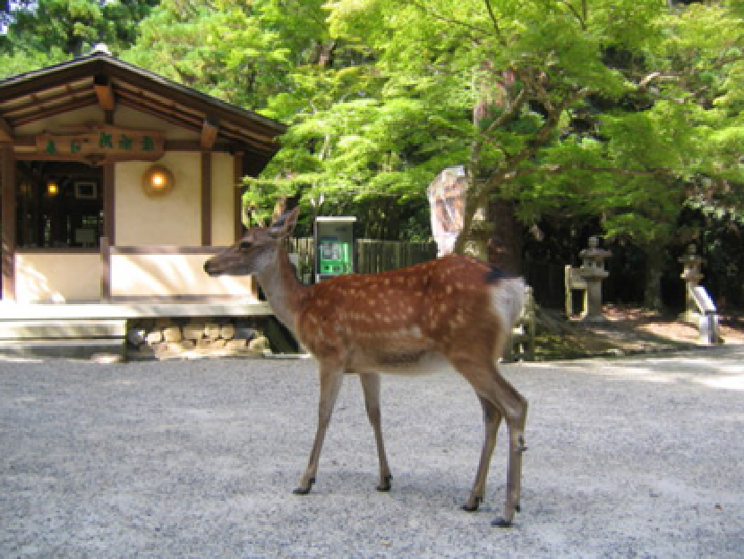
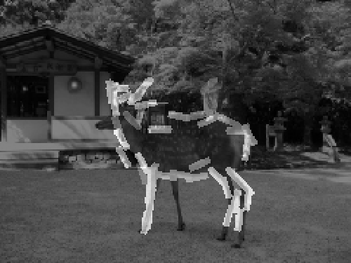
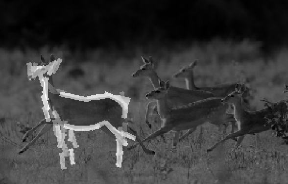
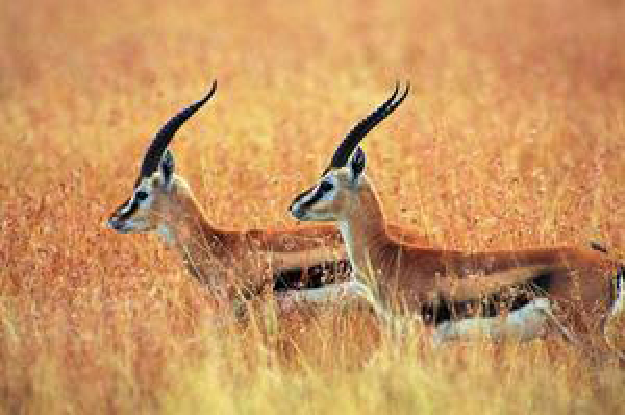
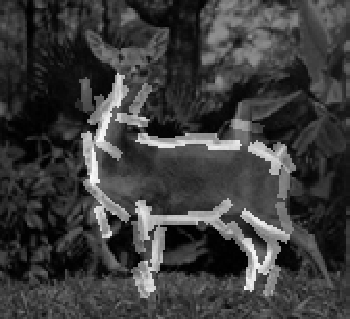
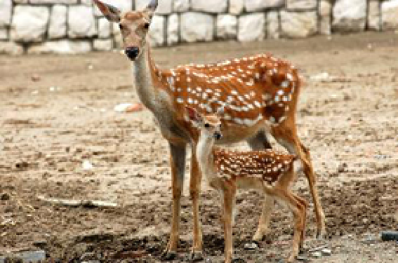
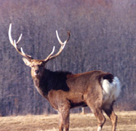
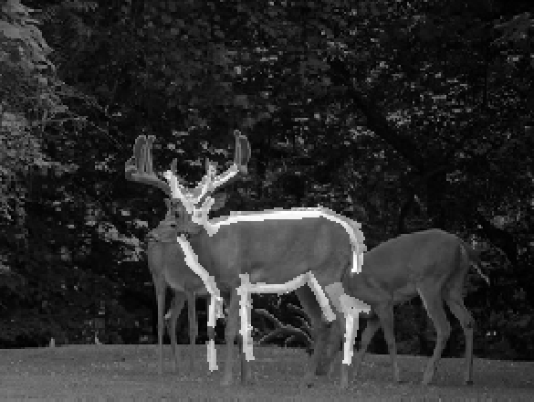
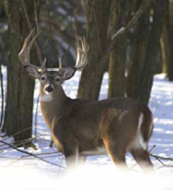
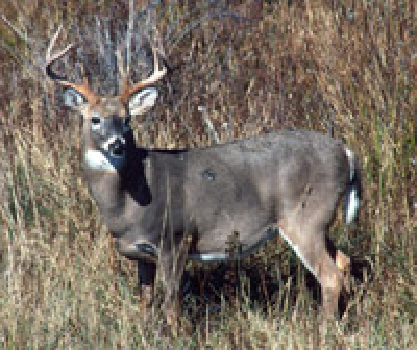
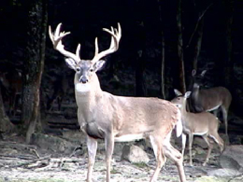
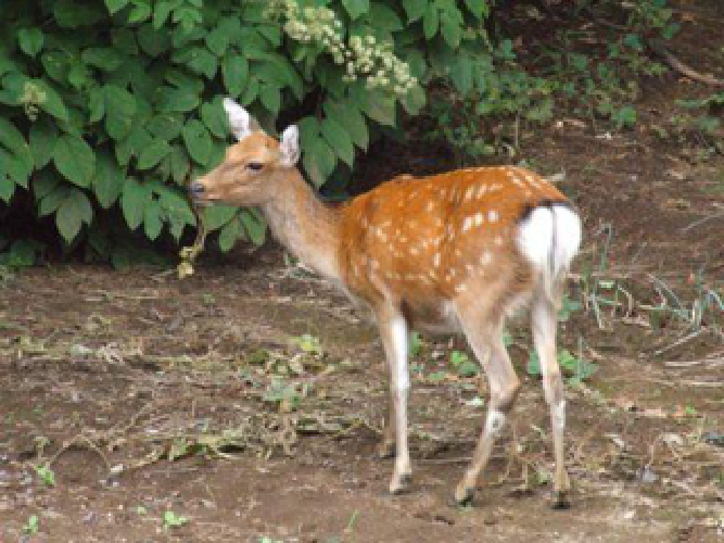
The 15 images are 179*112. Number of elements is 50.
eps
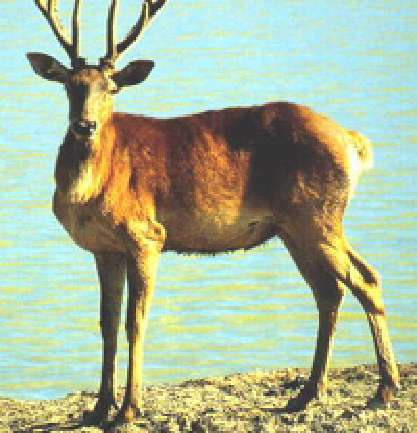
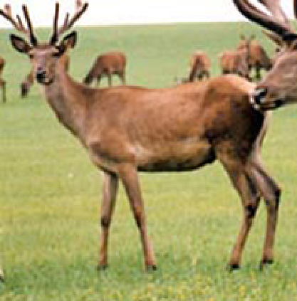
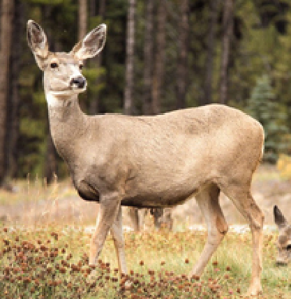
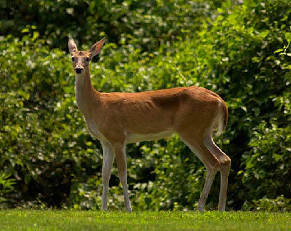
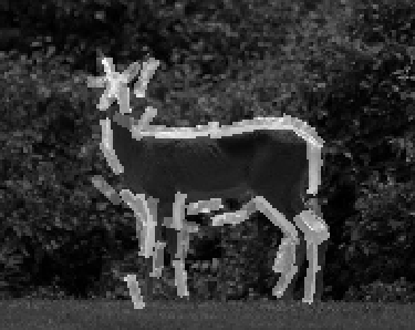
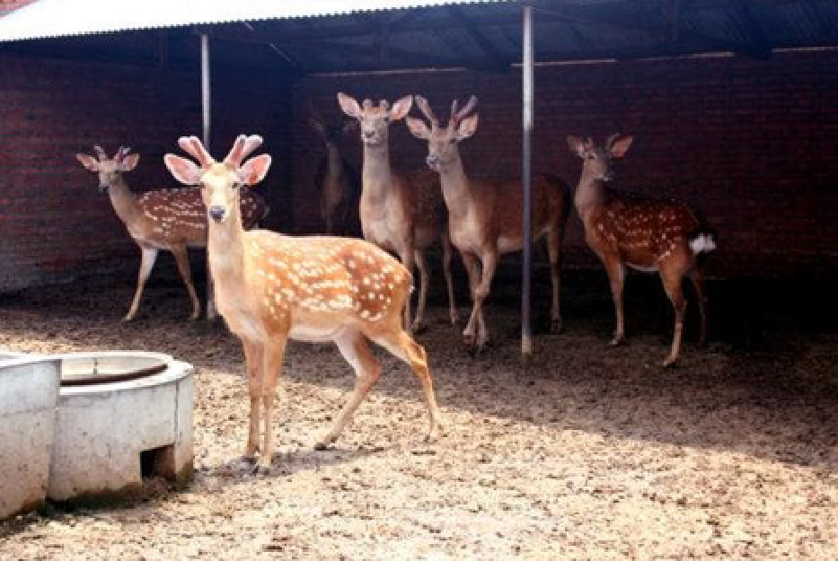
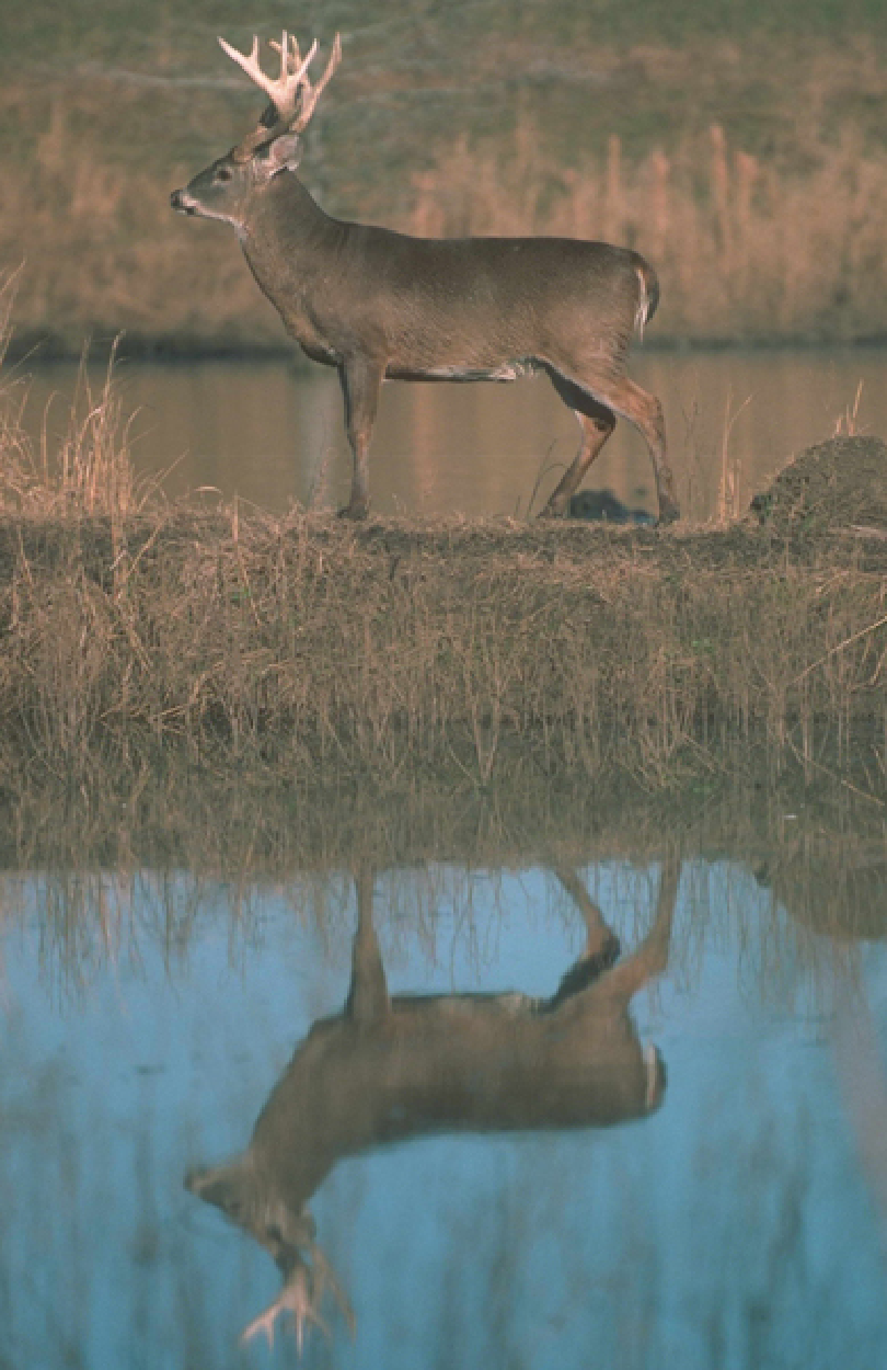
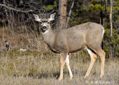
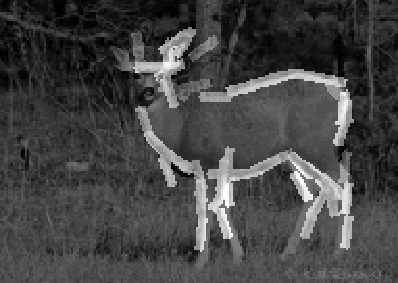
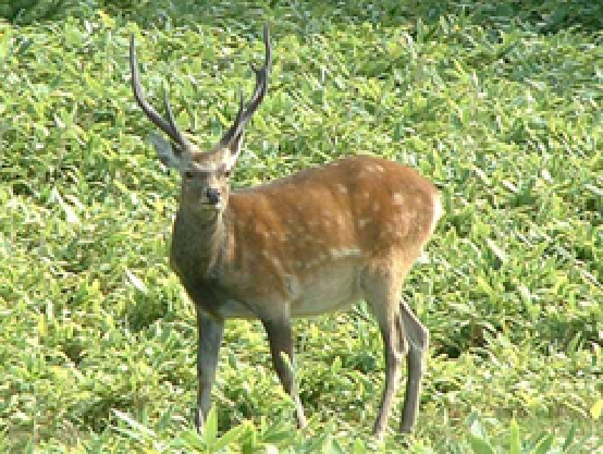
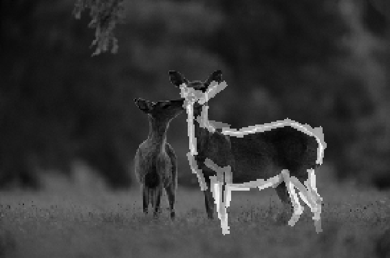
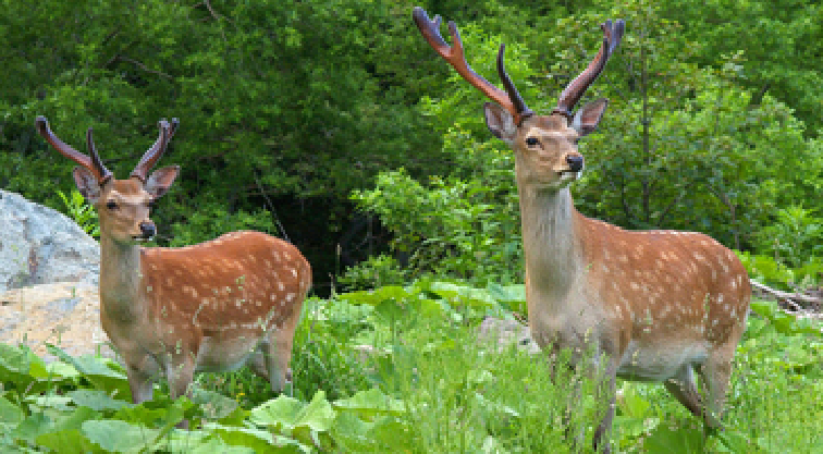
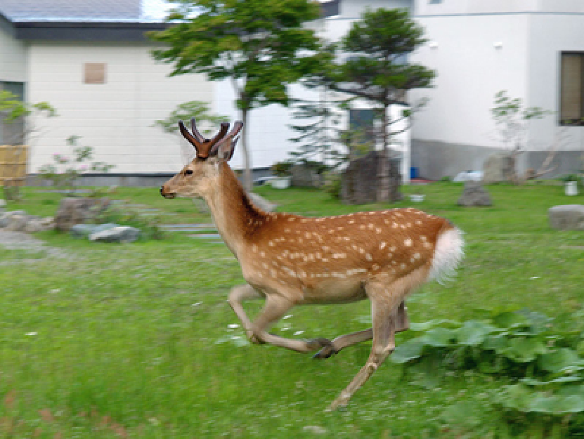
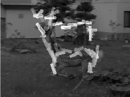
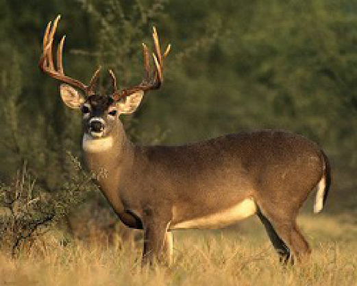
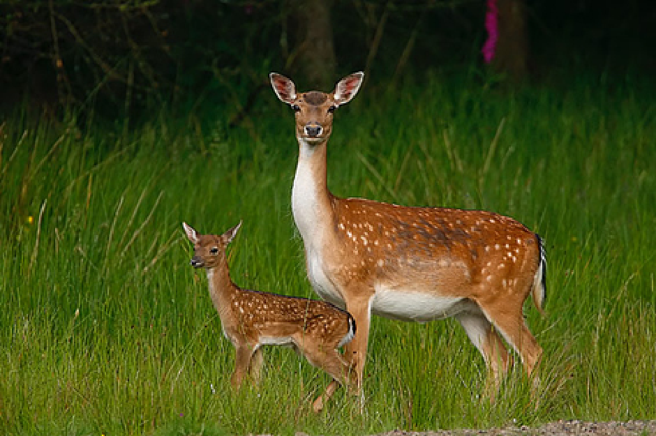
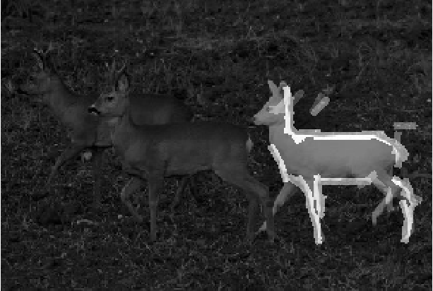
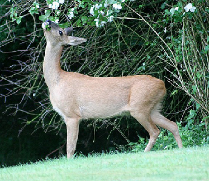
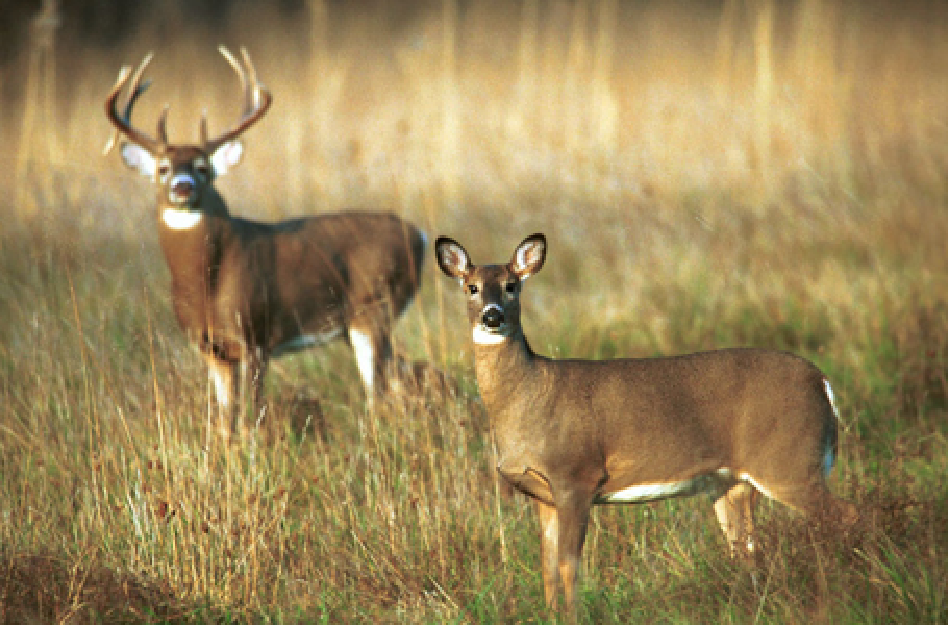
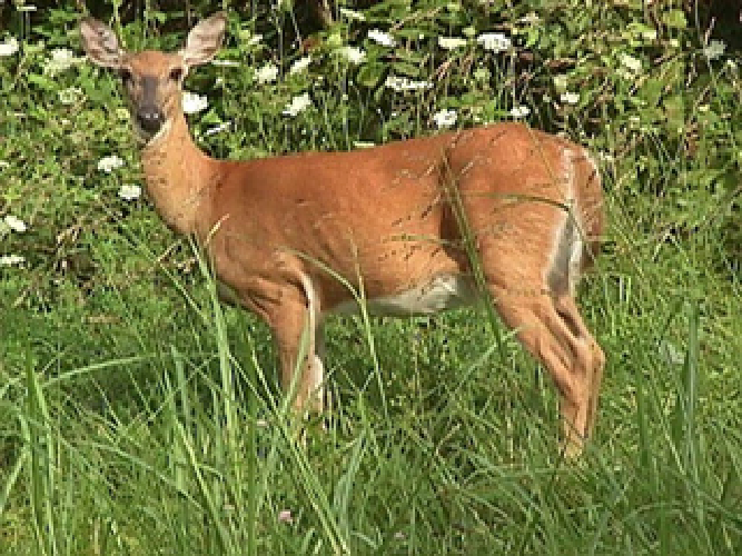
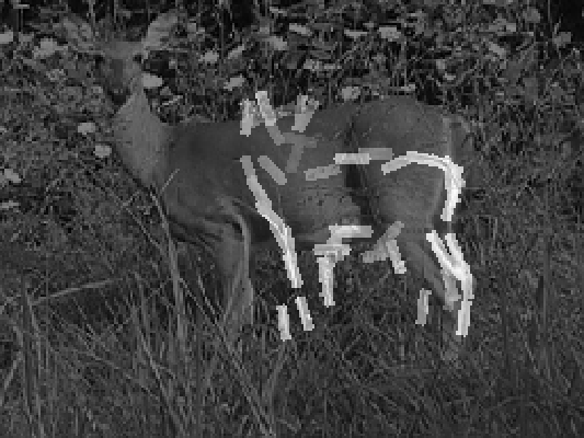
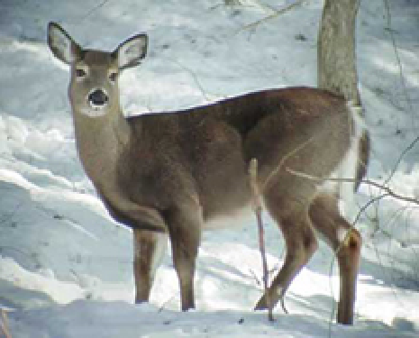
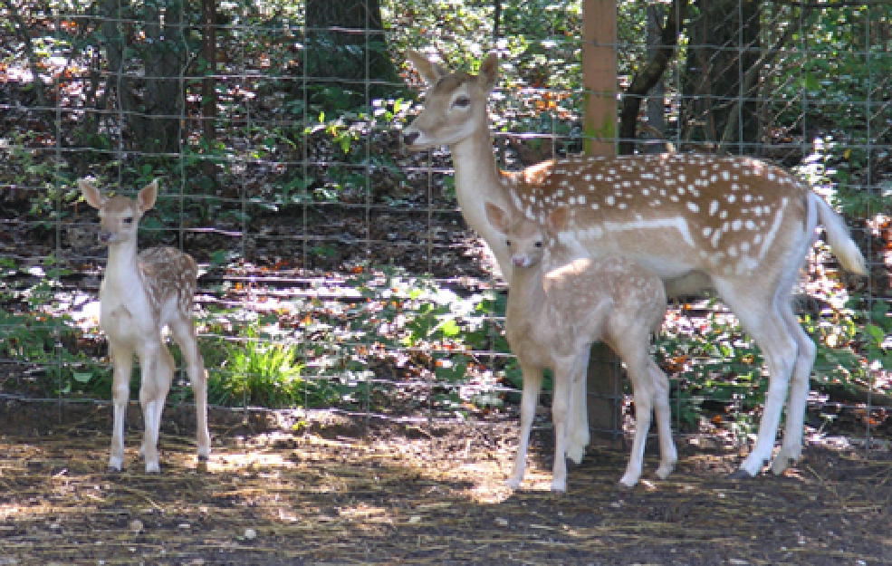
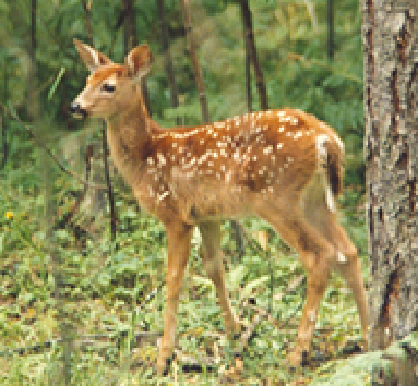
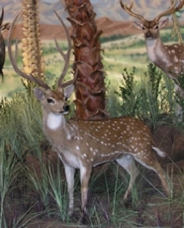
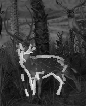
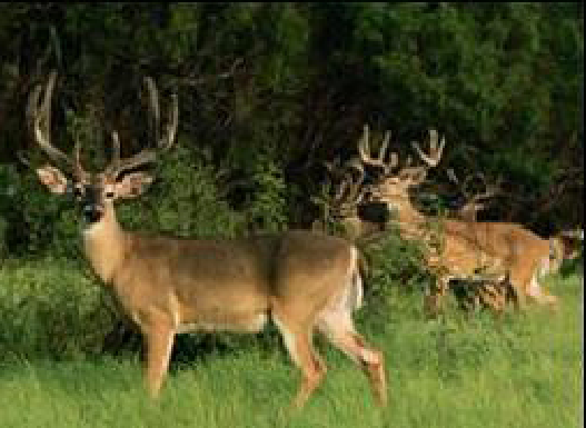
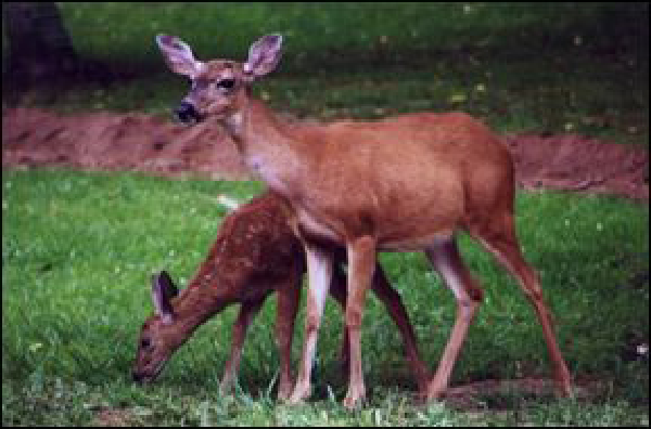
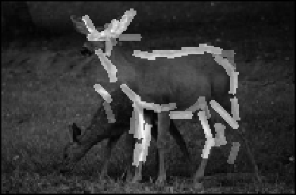
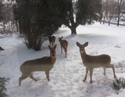
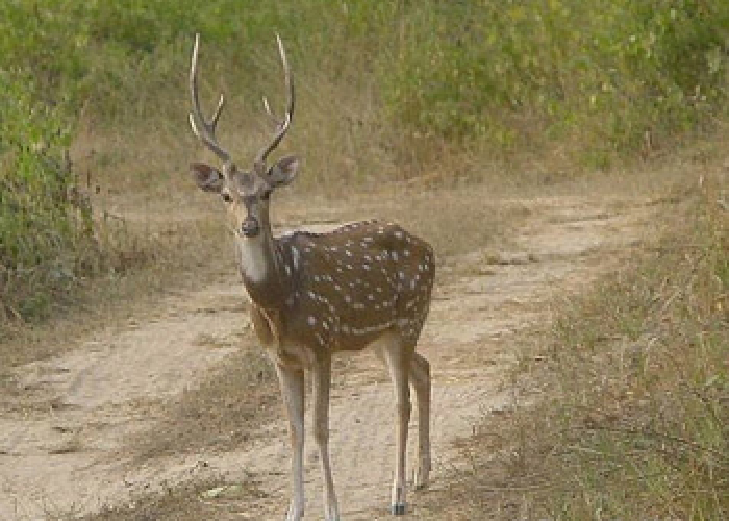
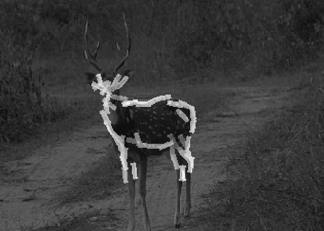
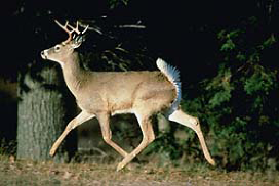
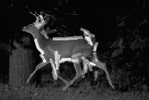
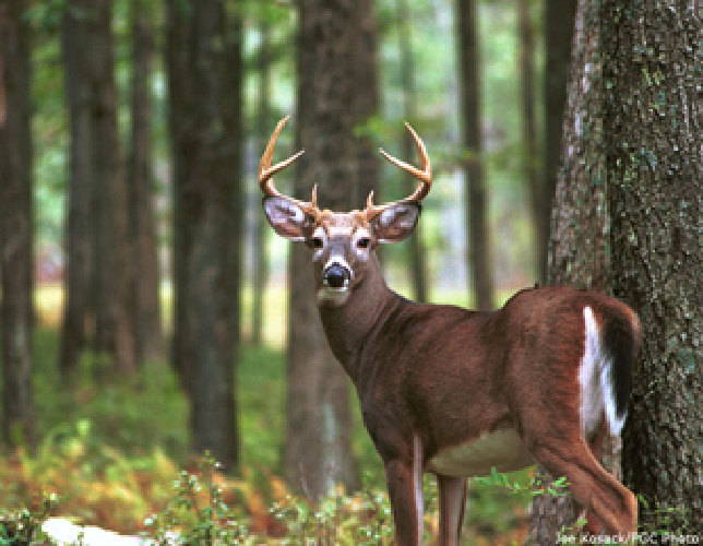
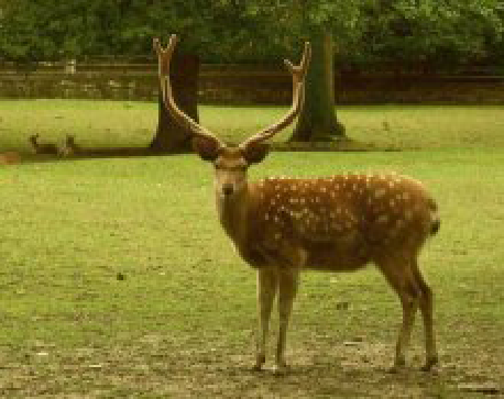
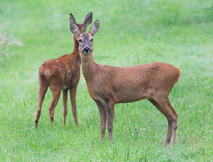
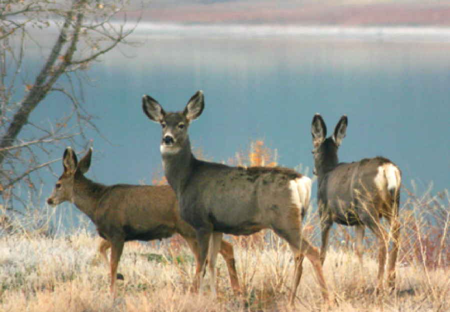
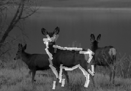
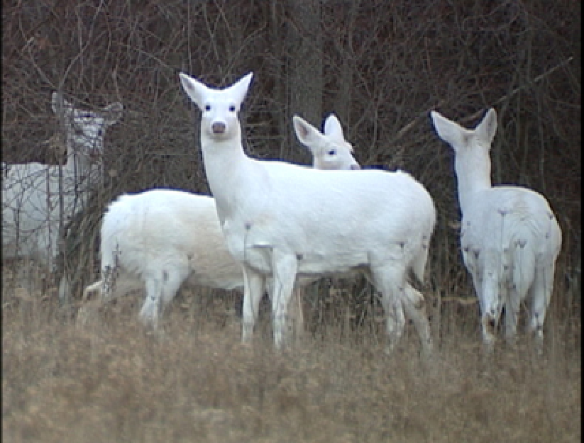
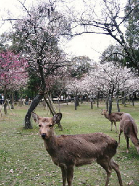
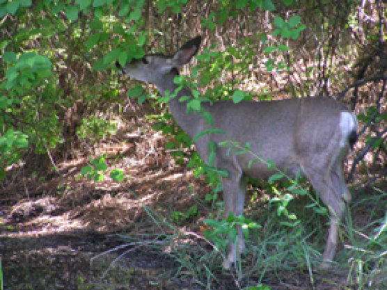
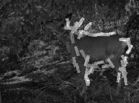
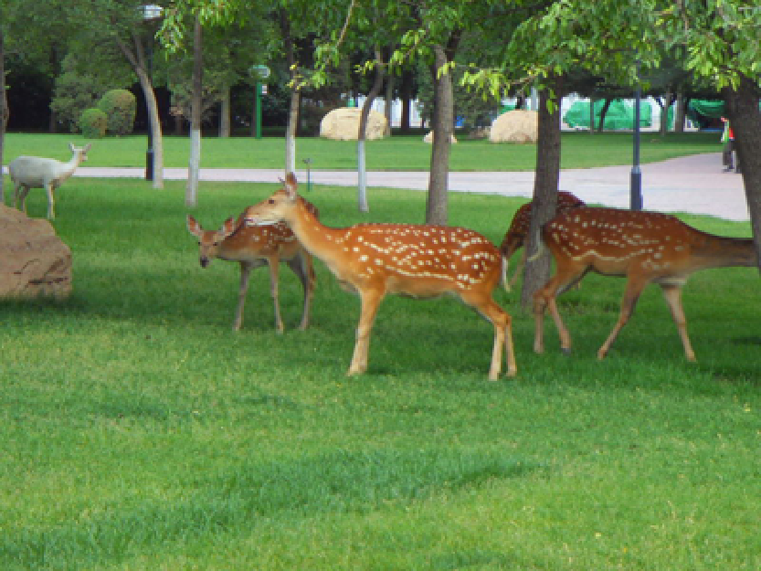
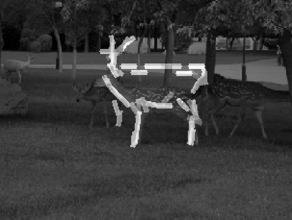
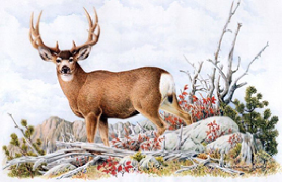
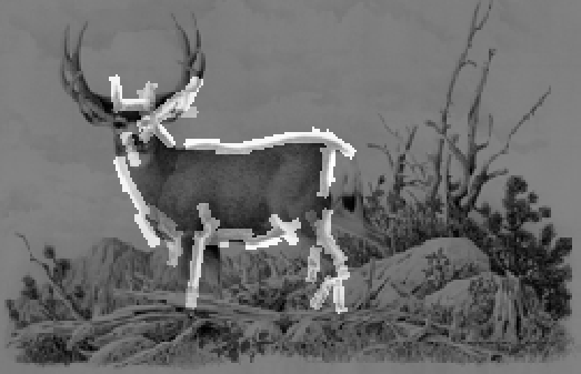
Testing image.
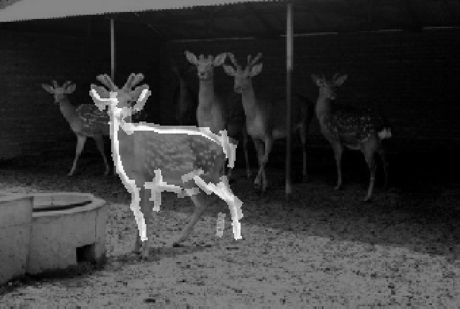
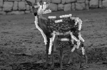
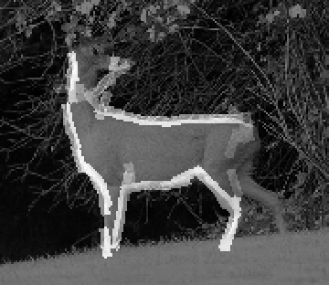
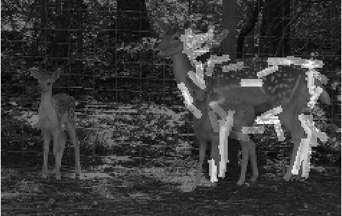
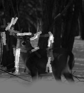
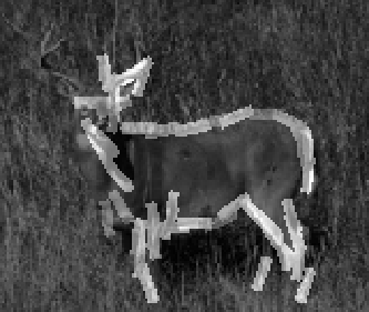
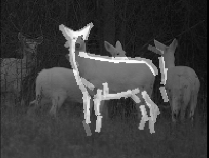
eps
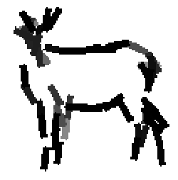
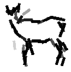
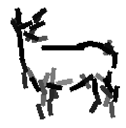
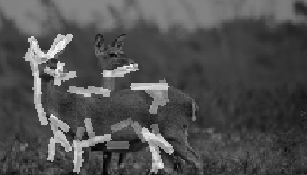
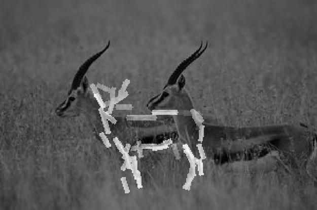
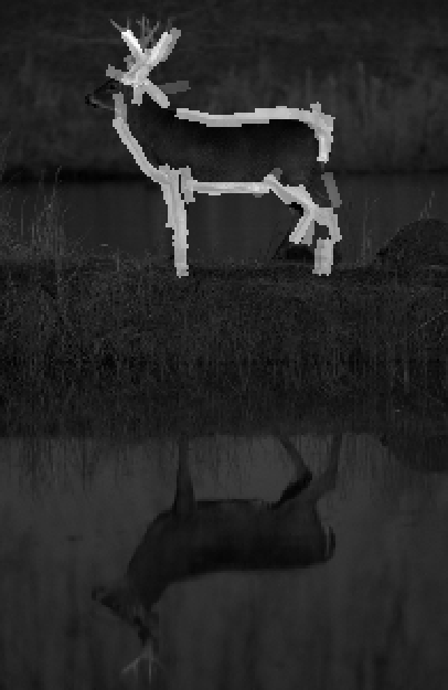
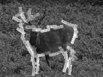
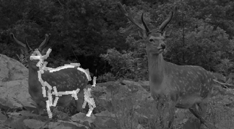
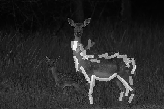
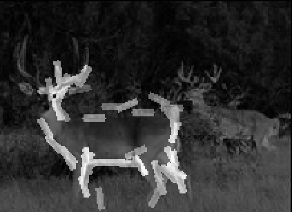
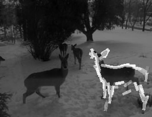
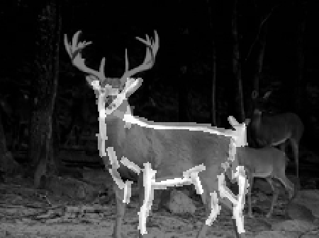
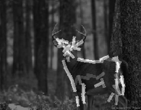
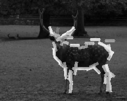
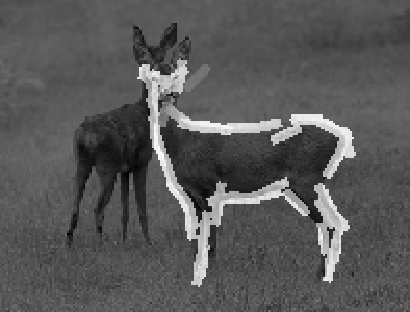
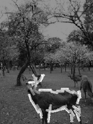
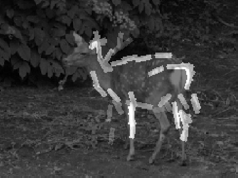
Superposed sketch of 50 elements of the deformed active basis
at each of the 10 resolutions, from 150*110 to 286*190. The bounding box is 179*112.
eps1
2
3
4
5
6
7
8
9
10
The MAX2 scores over ten resolutions.
eps
(2.2) code
with local normalization, half size of local window is 20. (August 2009)
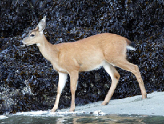
The 15 images are 179*112. Number of elements is 50.
eps

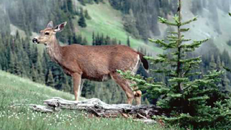
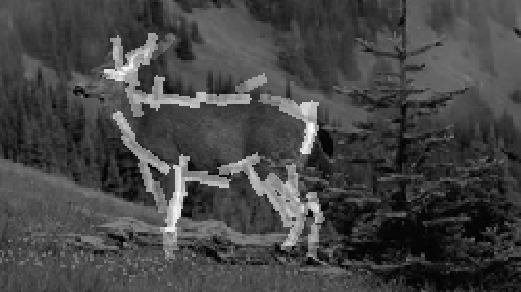
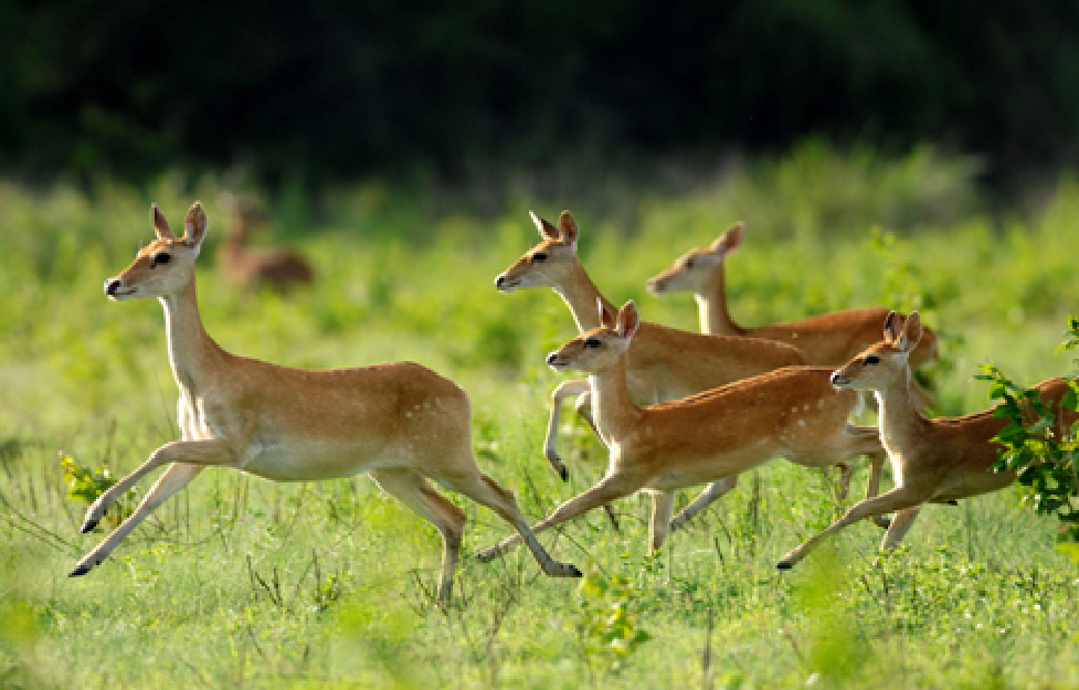
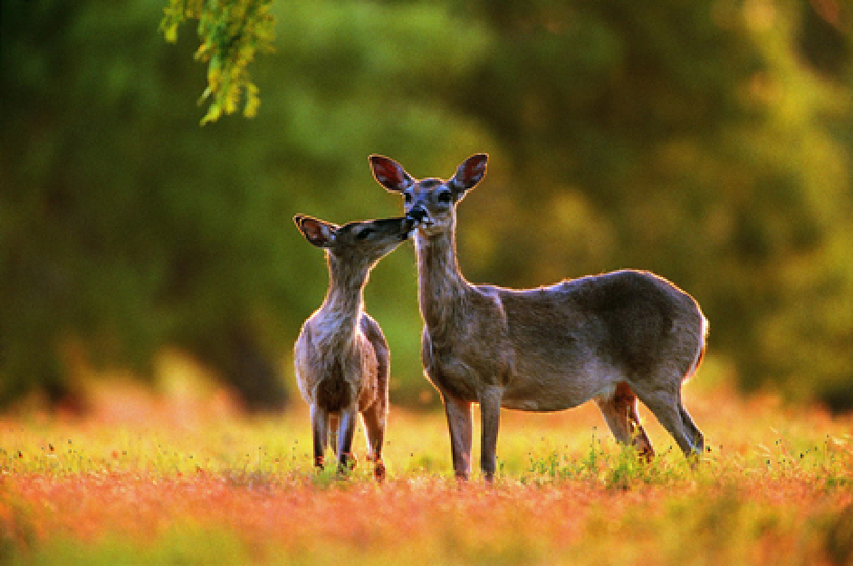
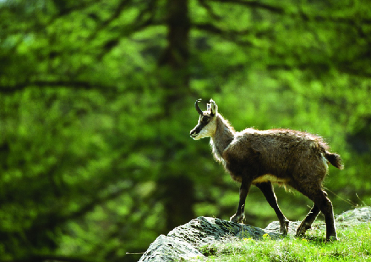
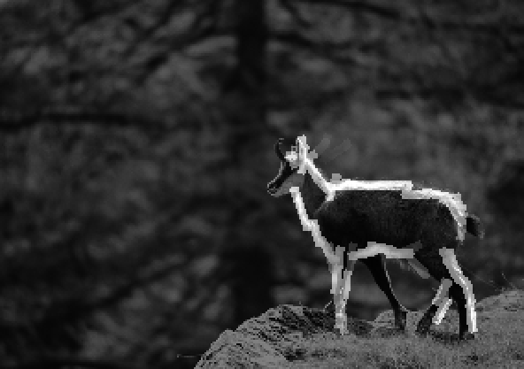
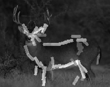
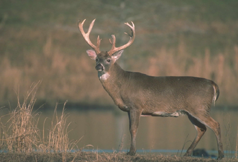
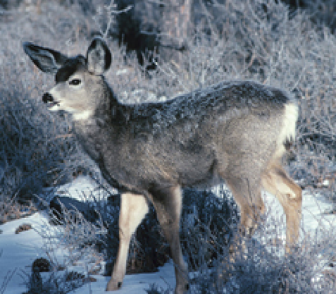
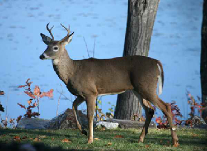
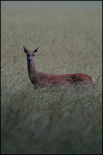
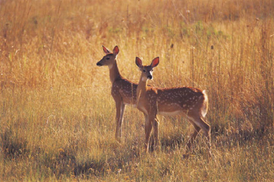
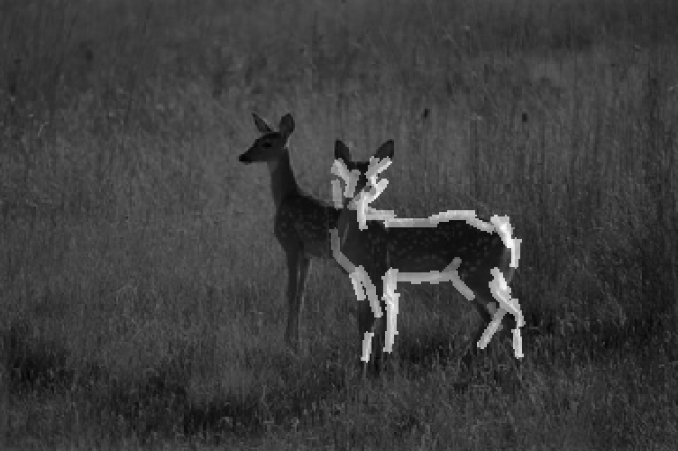
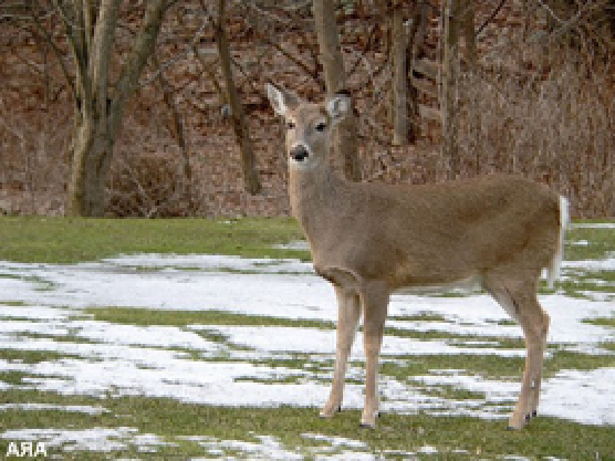
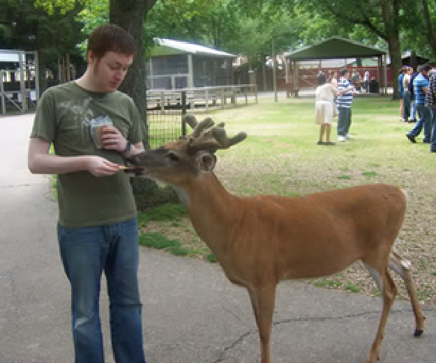
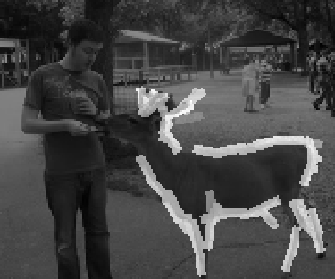
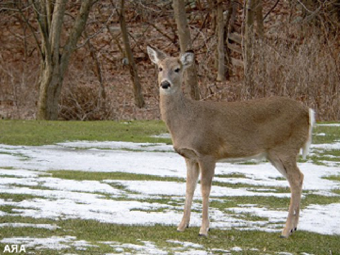
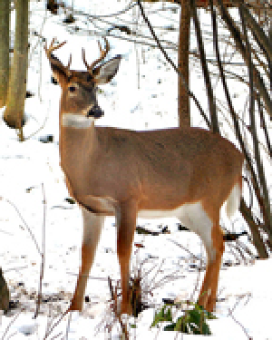
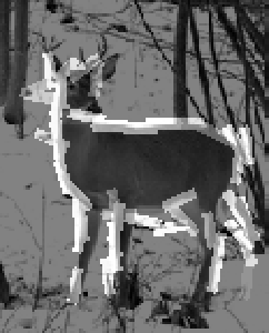
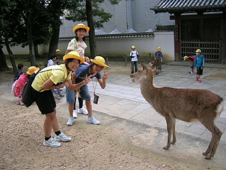
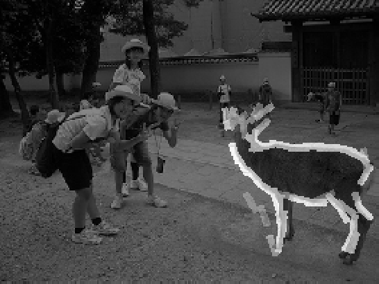
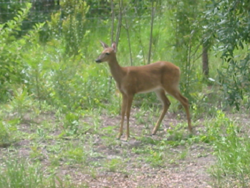
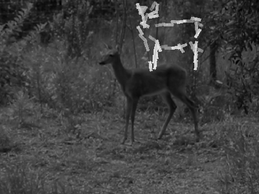
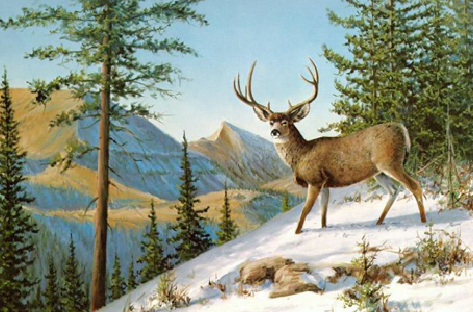
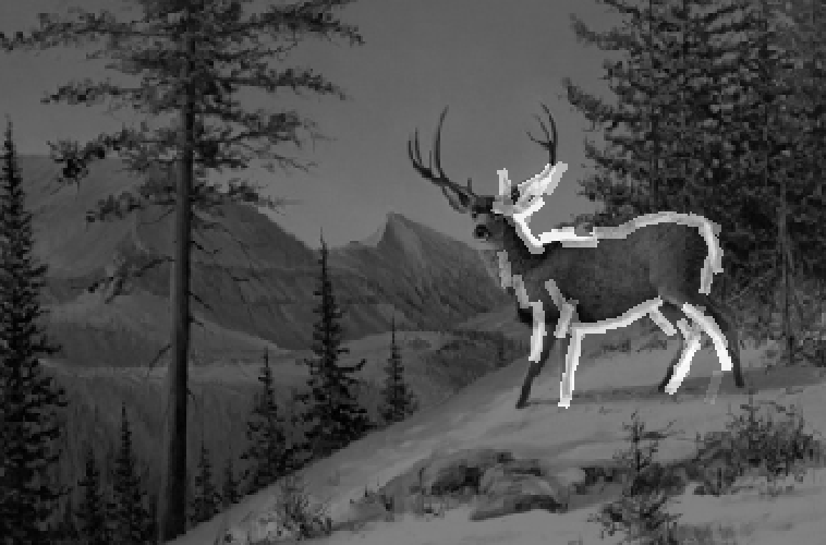
Testing image.
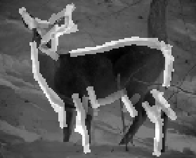
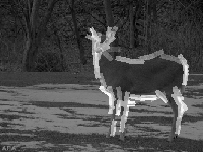
eps
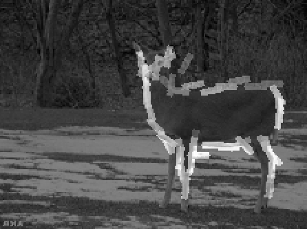
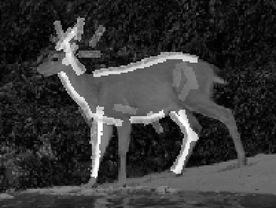
Superposed sketch of 50 elements of the deformed active basis
at each of the 10 resolutions, from 150*110 to 286*190. The bounding box is 179*112.
eps1
2
3
4
5
6
7
8
9
10
The MAX2 scores over ten resolutions.
eps
(2.2a) code
with local normalization, half size of local window is 20. (October 2009)
Testing image.
eps


Superposed sketch of 50 elements of the deformed active basis
at each of the 17 resolutions.
eps1
2
3
4
5
6
7
8
9
10
11
12
13
14
15
16
17
The MAX2 scores over 17 resolutions.
eps
(2.3) code
with local normalization (January 2010) data source: internet
scale = .7, half size of local window is 20. Number of elements is 50.
eps
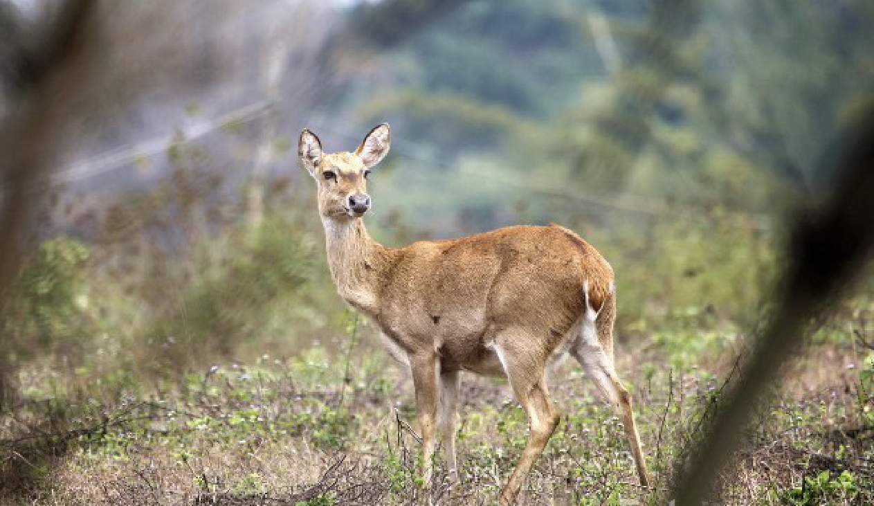
Testing image.
eps

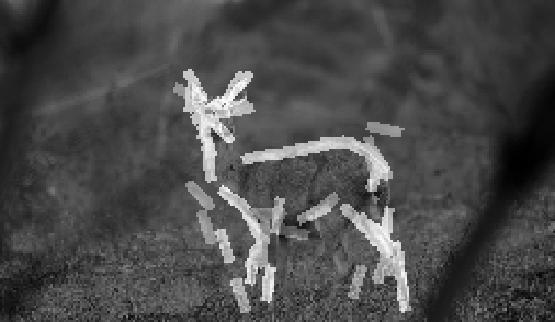
Superposed sketch of 50 elements of the deformed active basis
at each of the 10 resolutions.
eps1
2
3
4
5
6
7
8
9
10
The MAX2 scores over ten resolutions.
eps
(3)
Data and code (2008) data source: internet
(3.1)
Code with sigmoid transformation (2008)
The 12 images are 120*167. Number of elements is 50.
eps
(4)
Data and code (2008) data source: internet
The 9 images are 122*120. Number of elements is 50.
eps
(4.1)
Code with multi-scale Gabors, sigmoid transformation, normalization
within scanning window.(May 2009)
(4.2) code
with sigmoid transformation, within-window normalization, with q() pooled
from 2 natural images. (June 2009)
 eps1
2
3
4
5
eps1
2
3
4
5
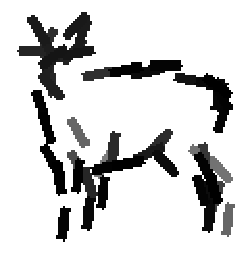
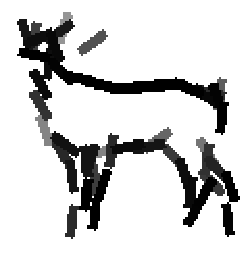
The learned templates with Gabors at 5 scales (.7, 1., 1.3, 1.6, 2.). Number of
elements at the smallest scale is 40. The numbers of elements at other scales are inverse
proportional to the corresponding scales.
 eps
eps
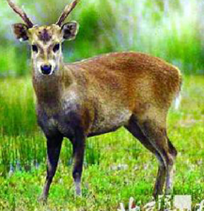
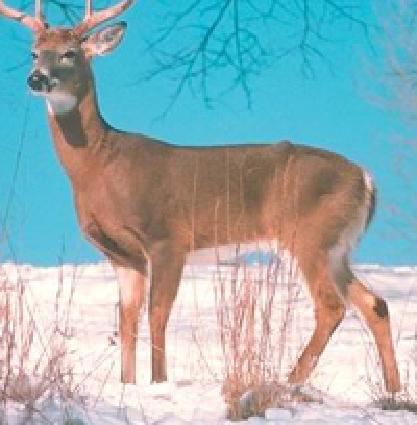
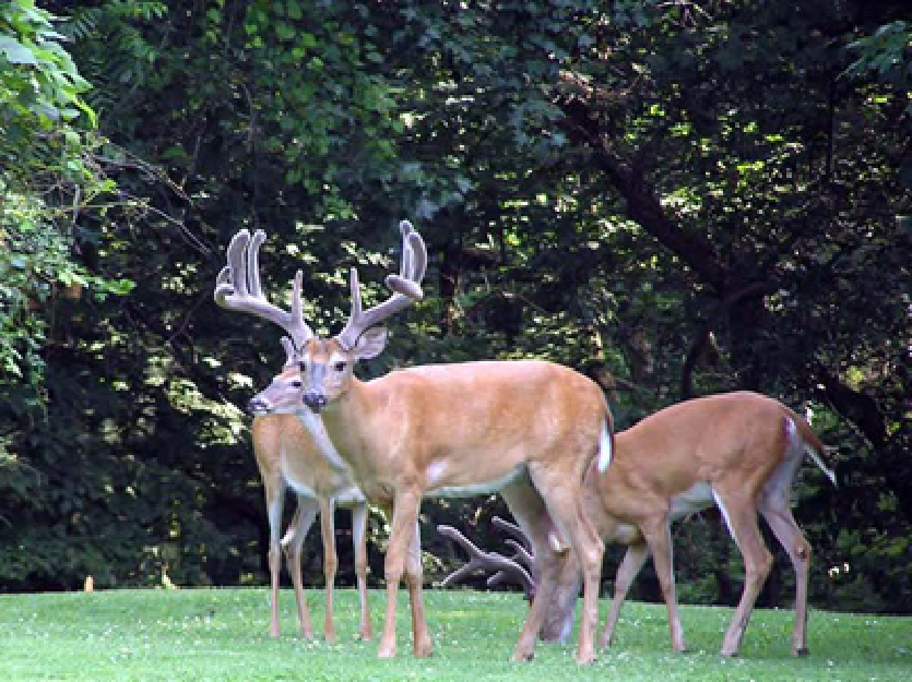
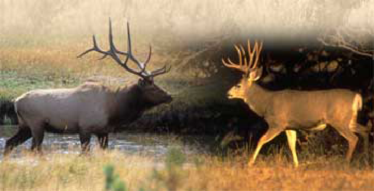
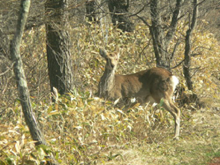
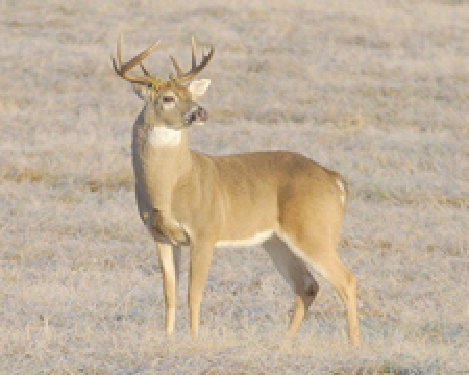
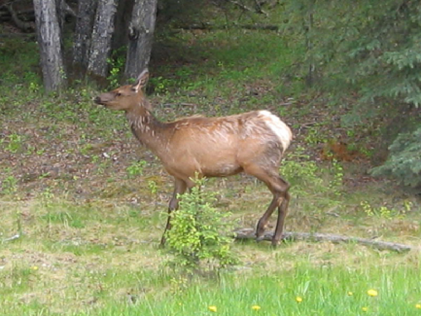
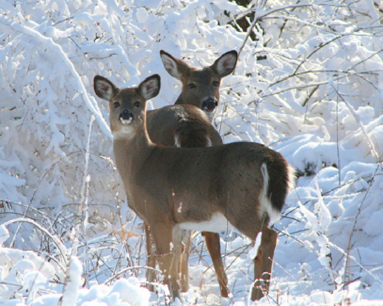
Testing image. We scan each template over 15 resolutions of the image,
from 110x140 to 341x434.
 eps1
2
3
4
5
eps1
2
3
4
5
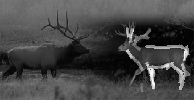
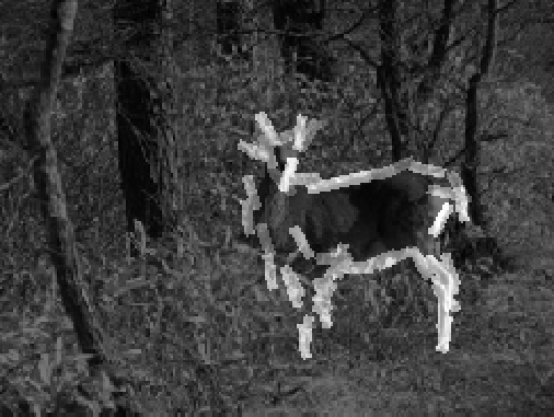
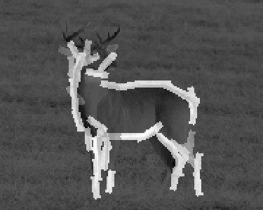
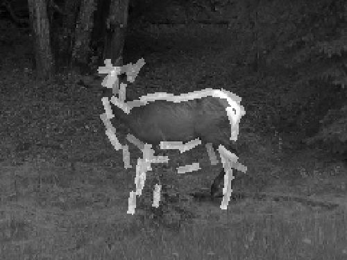
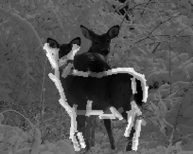
The superposed templates at 5 scales. Detection is
based on the SUM2 map that combines the scores of the 5 learned templates.
The MAX2 scores (combined over templates at 5 scales) over 15
resolutions of the image.
eps
The SUM2 map (combined over templates at 5 scales) at the optimal
resolution.
eps
(4.3) code
with sigmoid transformation, local normalization, with q() pooled
from 2 natural images. (June 2009)
using local normalization of filter responses. The haf size of
the local window is 20 pixels. Number of elements is 40.
eps
(5)
Data and code (2008) data source: internet
The 11 images are 133*140. Number of elements is 50.
eps
(6)
Data and code (March 2009) data source: Lotus Hill Institute

The images are 127x85. Number of elements is 30.
eps
The images are 150x100. Number of elements is 50.
eps
(7)
Data and code (August 2009) data source: internet
Scale is .7. Local normalization within a 41x41 neighborhood.
eps
(8)
Data and code (November 2009) data source: Lotus Hill Institute
Scale is 1. Local normalization within a 41x41 neighborhood.
eps
(9)
Data and code (November 2009) data source: Lotus Hill Institute
Scale is .7. Local normalization within a 41x41 neighborhood.
eps
(10)
Data and code (November 2009) data source: Lotus Hill Institute
Scale is .7. Local normalization within a 41x41 neighborhood.
eps
(11)
Data and code (January 2010) data source: Lotus Hill Institute
Scale is .7 Local normalization within a 41x41 neighborhood.
eps
(12)
Data and code (January 2010) data source: Lotus Hill Institute
Scale is .7 Local normalization within a 41x41 neighborhood.
eps
(13)
Data and code data source: Lotus Hill Institute
Scale is .7 Local normalization within a 43x43 neighborhood.
eps
(14)
Data and code data source: Caltech 101
Number of training images = 58; Number of elements = 60;
Length of Gabor = 17 pixels; Range of displacement = 4 pixels;
Subsample rate = 1 pixel; Image height and width = 88 by 143 pixels.
eps
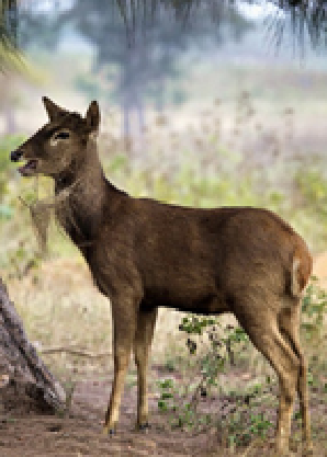
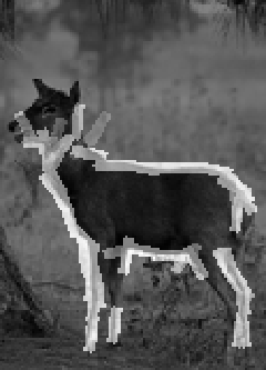
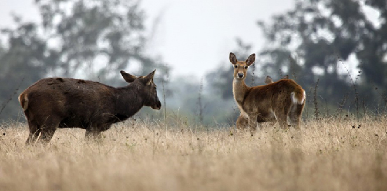
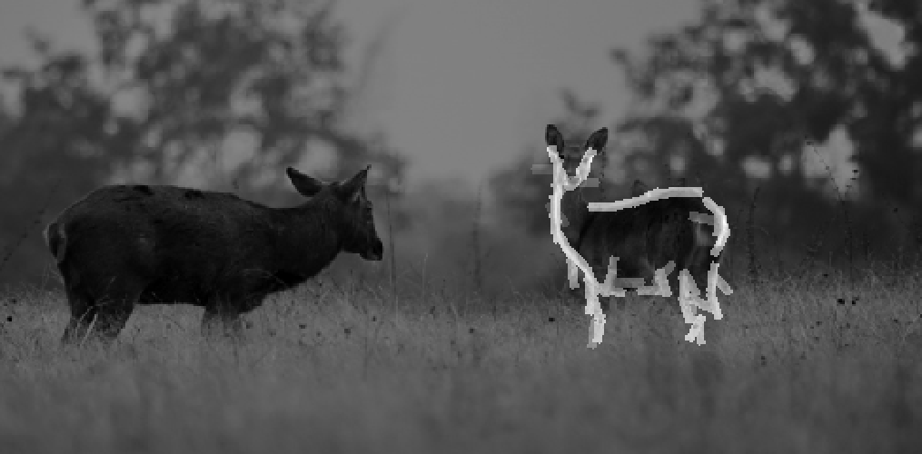
(15)
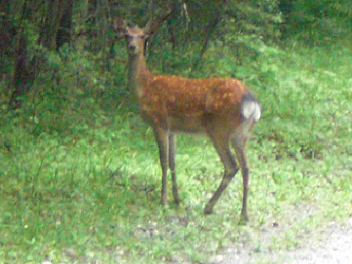
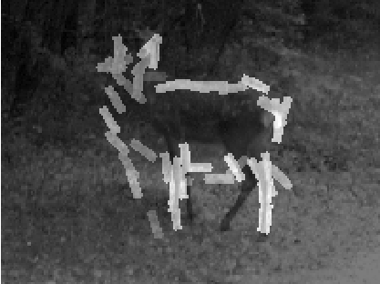
Data and code data source: LHI
Number of training images = 60; Number of elements = 50;
Length of Gabor = 17 pixels; Range of displacement = 4 pixels;
Subsample rate = 1 pixel; Image height and width = 120 by 120 pixels
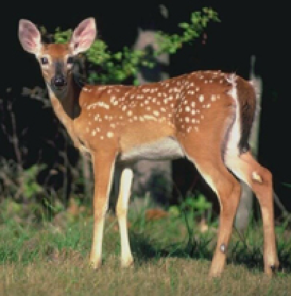
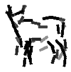
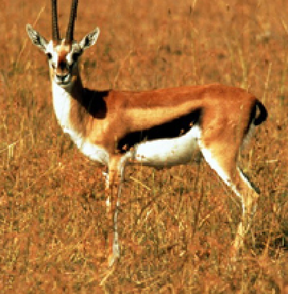
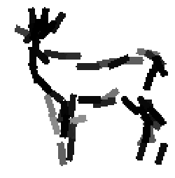
Things can be difficult on Serengeti because of textures.
It appears that local normalization of filter responses is better
than normalization within the template window for such images.
Currently, we let the half size of the local window to be roughly
the same as the length of the Gabor element.
(16)
Zebra (August 2009) data source: internet
Scale is 1.5. Number of elements is 35. Local normalization within
a 61x61 neighborhood.
eps
(17)
Giraff (August 2009) data source: internet
Scale is 1.0. Number of elements is 40. Local normalization within
a 41x41 neighborhood.
eps
(18)
Elephant (August 2009) data source: internet
Scale is 1.0. Local normalization within a 41x41 neighborhood.
eps
(19)
Elephant front view (August 2009) data source: internet
Scale is 1.0. Local normalization within a 41x41 neighborhood.
eps
(20)
Lion (August 2009) data source: internet
Scale is 1.0. Local normalization within a 41x41 neighborhood.
eps
(21)
Bear (August 2009) data source: internet
Scale is 1.0. Local normalization within a 41x41 neighborhood.
eps
Poor man version (December, 2009)
Inhibition is done on the pooled MAX1 maps, instead of over
individual SUM1 maps. This can save a lot of computing time,
especially used in EM loops. But the learned template can be
less clean.
Back to active basis homepage