International Journal of Computer Vision
Learning Sparse FRAME Models for Natural Image Patterns
Jianwen Xie 1 Wenze Hu 2 Song-Chun Zhu 1 Ying Nian Wu 1
1 University of California, Los Angeles (UCLA), USA 2 Google Inc, USA
Abstract |
|
It is well known that natural images admit sparse representations by redundant dictionaries of basis functions such as Gabor-like wavelets. However, it is still an open question as to what the next layer of representational units above the layer of wavelets should be. We address this fundamental question by proposing a sparse FRAME (Filters, Random field, And Maximum Entropy) model for representing natural image patterns. Our sparse FRAME model is an inhomogeneous generalization of the original FRAME model. It is a non-stationary Markov random field model that reproduces the observed statistical properties of filter responses at a subset of selected locations, scales and orientations. Each sparse FRAME model is intended to represent an object pattern and can be considered a deformable template. The sparse FRAME model can be written as a shared
sparse coding model, which motivates us to propose a twostage algorithm for learning the model. The first stage selects the subset of wavelets from the dictionary by a shared matching pursuit algorithm. The second stage then estimates the parameters of the model given the selected wavelets. Our experiments show that the sparse FRAME models are capable of representing a wide variety of object patterns in natural images and that the learned models are useful for object classification.
|
1. Inhomogeneous FRAME
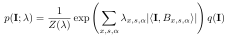
1.1 Model
|
1.2 Learning
The FRAME model is a special case of the exponential family model, and the parameter λ={λx,s,α, ∀x,s,α} can be estimated from the training images by MLE.
The MLE can be obtained by the stochastic gradient algorithm analyzed by Younes (1999) [1]. Let λ(t) be the current estimate of λ, and let {![]() m, m = 1,...,
m, m = 1,...,![]() } be a sample of synthesized images drawn from p(I; λ(t) ). Then we can update λ by
} be a sample of synthesized images drawn from p(I; λ(t) ). Then we can update λ by
|
where![]() is the step size. The synthesized images {
is the step size. The synthesized images {![]() m, m = 1,...,
m, m = 1,...,![]() } can be drawn from p(I; λ(t) ) by Hamiltonian Monte Carlo (HMC) [2]. The ratio of the normalizing constants
} can be drawn from p(I; λ(t) ) by Hamiltonian Monte Carlo (HMC) [2]. The ratio of the normalizing constants
|
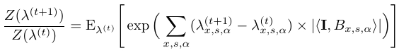
can be approximated by averaging over the sampled images
{![]() m}. Starting from λ(0) = 0 and log Z(λ(0)) = 0, we can
compute log Z(λ(t)) along the learning process by iteratively updating
its value as follows:
m}. Starting from λ(0) = 0 and log Z(λ(0)) = 0, we can
compute log Z(λ(t)) along the learning process by iteratively updating
its value as follows:
|
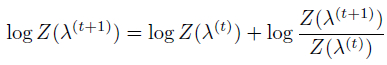
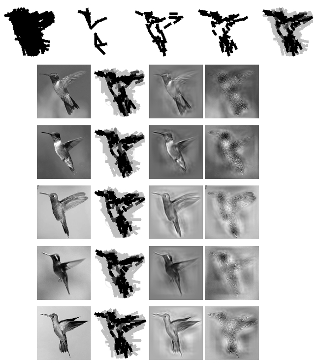
Figure 2 illustrates the learning process by showing the synthesized images with λ being updated by the algorithm. The synthesized image starts from Gaussian white noises sampled from q(I), then gradually gets similar to the observed images in the overall shape and appearance.
|


2. Sparse FRAME
2.1 Model
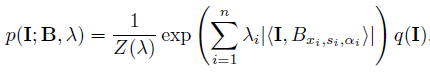
In model (1), the (x,s,α) in ![]() x,s,α is over all the pixels x and all the scales s and orientations α. We call such a model the dense FRAME. It is possible to sparsify the model by selecting only a small set of (x,s,α) so that
x,s,α is over all the pixels x and all the scales s and orientations α. We call such a model the dense FRAME. It is possible to sparsify the model by selecting only a small set of (x,s,α) so that ![]() x,s,α is restricted to this selected subset, while such a selected subset of basis functions should be enough to interpret or reconstruct the training images. More explicitly, we can write the sparsified model as
x,s,α is restricted to this selected subset, while such a selected subset of basis functions should be enough to interpret or reconstruct the training images. More explicitly, we can write the sparsified model as
|
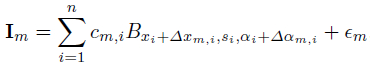
where n is the number of selected basis function, λ={λi, i=1,...,n} are the coefficients, and { Bxi,si,αi , i=1,...,n} is the selected set of basis functions shared by training images. We may allow these shared basis functions to perturb their locations and orientations to account for shape deformations. (Δxm,i , Δαm,i) are the perturbations of the location and orientation of the i-th basis function in the m-th image. Both Δxm,i and Δαm,i are assumed to vary within limited ranges.
2.2 Learning
The learning algorithm consists of two stages. (1) Selecting B = {Bxi,si,αi , i=1,...,n} by deformable shared sparse coding. (2) Estimating λ={λi, i=1,...,n} given selected B.
Stage 1: We want to select the basis functions B = {Bxi,si,αi , i=1,...,n} by minimizing the sum of reconstruction errors of all training images
|
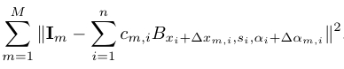
We can extend the matching pursuit algorithm [3] to select basis functions to code multiple images simultaneously, while inferring local perturbations by local max pooling [4]:
Deformable shared matching pursuit algorithm
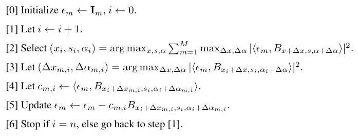
Stage 2 : After selecting B = {Bxi,si,αi , i=1,...,n}, we can then model {Im} by the sparse FRAME model (6), by estimating λ at MLE. p(I; B, λ) in (6) now served as the deformable template in that the log-likelihood ratio of the Im is
|
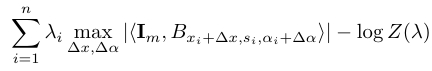
which serves as the template matching score, where we allow
each selected Bi to perturb its location and orientation in view of (5), with the perturbations inferred by local max
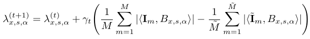
pooling. Again, let λ(t) be the current estimate of λ, and let {![]() m, m = 1,...,
m, m = 1,...,![]() } be the synthesized images drawn from p(I; λ(t) ) by
} be the synthesized images drawn from p(I; λ(t) ) by ![]() parallel chains. Then we can update λ by
parallel chains. Then we can update λ by
|
The learned p(I; λ(t) ) models the appearance of the undeformed template. So there is an explicit separation between appearance and shape variations.After we learn λ and compute Z(λ) as in (4), we can use the learned model as a deformable template to be matched to the testing image, where the template matching score at each location can be computed like (8).
|
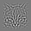
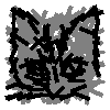
3. Synthesis by FRAME
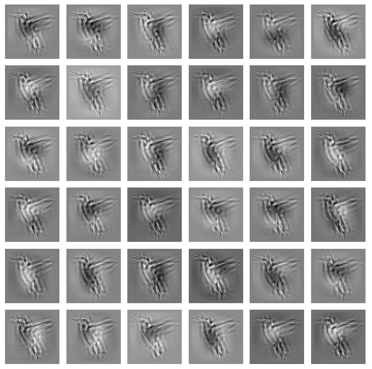
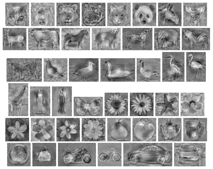
Figure 5 and Figure 6 displays some images generated by the dense models and the sparse models learned from roughly aligned training images respectively. All the synthesized images are generated by the HMC algorithm along the learning process.
|
4. Geometric Transformation
We can obtain the geometrically transformed versions of the learned model by directly applying the operations of dilation, rotation, flipping, or even changing the aspect ratio to B = {Bxi,si,αi , i=1,...,n} without changing the values of λ. This amounts to simple affine transformations of (xi,si,αi, i=1,...,n). Figure 7 shows some examples of geometric transformations of the sparse FRAME model: flipping and rotation.
|
||||||
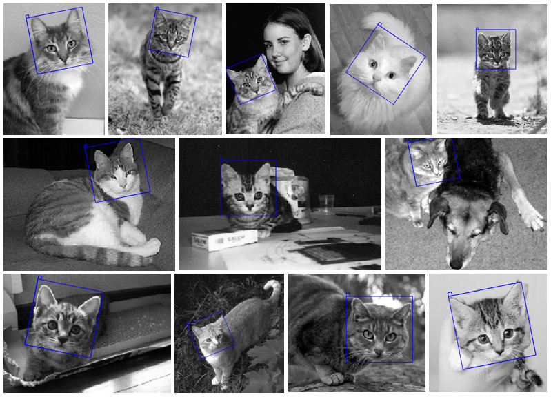
5. Detection
The learned model can be used to detect the object in a testing image by deformable template matching. We can scan the template over the image domain D, and at each location X ∈ D, we match the template to the image patch within the bounding box centered at X by computing the template matching score based on (8). We then choose the location X that achieves the maximum template matching score as the center of the detected object. We also allow geometric transformation of template in detection, which includes rotation, scaling and left-right flipping. Figure 8 shows examples of detection.
|
||||
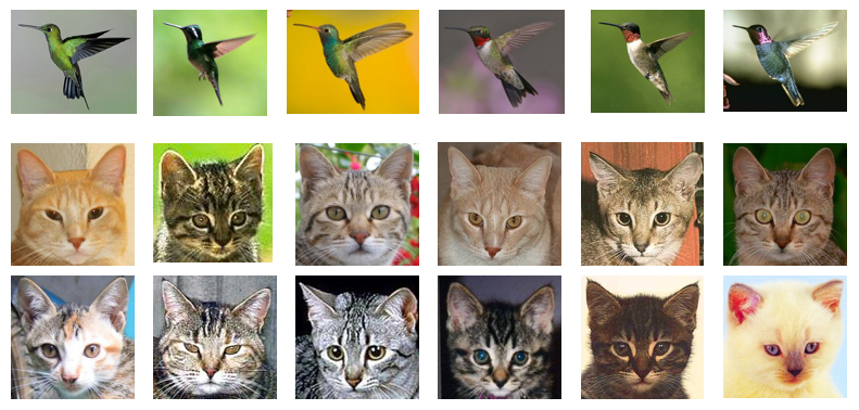
6. Clustering
Model-based clustering can be accomplished by EM-type algorithm that fits mixtures of sparse FRAME models. Figure 9 and Figure 10 illustrate 5 experiments. The EM-type algorithm usually converges within 3-5 iterations. For each cluster, we generate 144 parallel chains in learning.
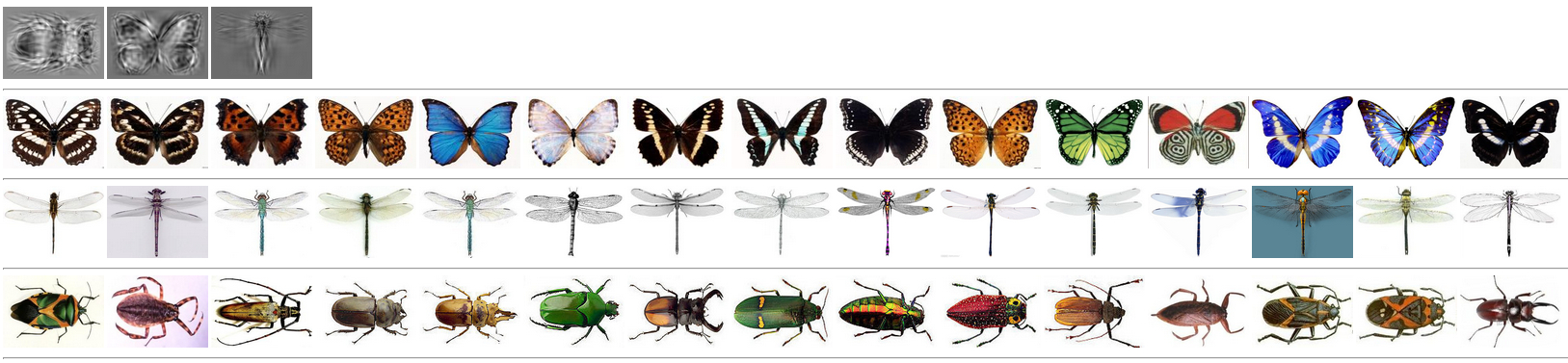
Fig 9. Clustering. First row: synthesized images from a mixture of sparse FRAME models learned from 45 training images. Last three rows: three groups of training images are separated by the mixture models. Number of wavelets in each model is 300.
To evaluate the clustering quality, we use two metrics: conditional purity and conditional entropy [5]. For a random training image, let x be its true category (unknown to the algorithm) and y be the infered category. The conditional purity is defined as
and the conditional entropy is defined as,
where both p(y) and p(x|y) can be estimated from the training set, and we would expect higher purity and lower entropy for a better clustering algorithm. We perform 7 clustering experiments. The number of clusters vary from 2 to 5 and are assumed known in these experiments. The number of images in each cluster is typically 15 except in one experiment. We compare the performance of the sparse FRAME with that of k-means based on HoG features. Table 1 displays the clustering accuracies and standard errors based on 10 repetitions of each experiment. |
Fig 10. Clustering. Each row illustrates one clustering experiment by displaying a synthesized image (100 × 100) and a training example from each cluster. Typical number of wavelets for each template is 300. The number of images within each cluster is around 15 to 20 images. |
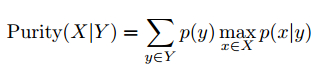
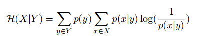
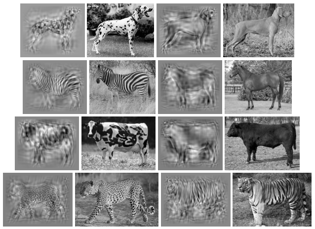
Table 1. Comparison of conditional purity (the first two rows) and conditional entropy (the last two rows) between sparse FRAME and k-means for clustering
Exp1 |
Exp2 |
Exp3 |
Exp4 |
Exp5 |
Exp6 |
Exp7 |
|
|---|---|---|---|---|---|---|---|
| k-means (purity) | 0.623 ± 0.016 |
0.870 ± 0.043 |
0.933 ± 0.141 |
0.825 ± 0.121 |
0.911 ± 0.086 |
0.888 ± 0.091 |
0.687 ± 0.110 |
| FRAME (purity) | 0.943 ± 0.063 |
0.990 ± 0.016 |
0.938 ± 0.131 |
0.895 ± 0.132 |
1.000 ± 0.000 |
0.879 ± 0.141 |
0.741 ± 0.111 |
| k-means (entropy) | 0.652 ± 0.009 |
0.376 ± 0.086 |
0.092 ± 0.195 |
0.243 ± 0.167 |
0.226 ± 0.084 |
0.199 ± 0.126 |
0.639 ± 0.161 |
| FRAME (entropy) | 0.145 ± 0.157 |
0.037 ± 0.060 |
0.090 ± 0.191 |
0.155 ± 0.189 |
0.000 ± 0.000 |
0.179 ± 0.208 |
0.497 ± 0.192 |
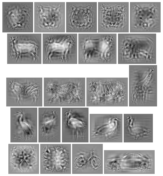
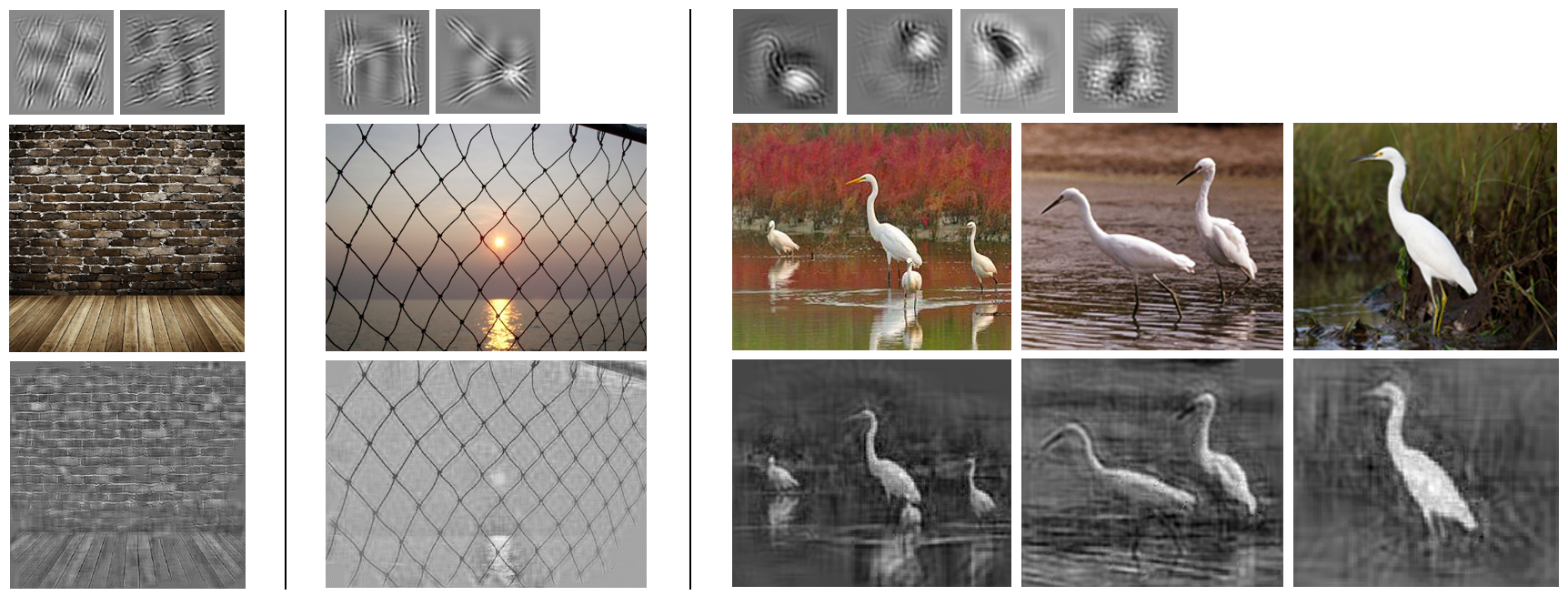
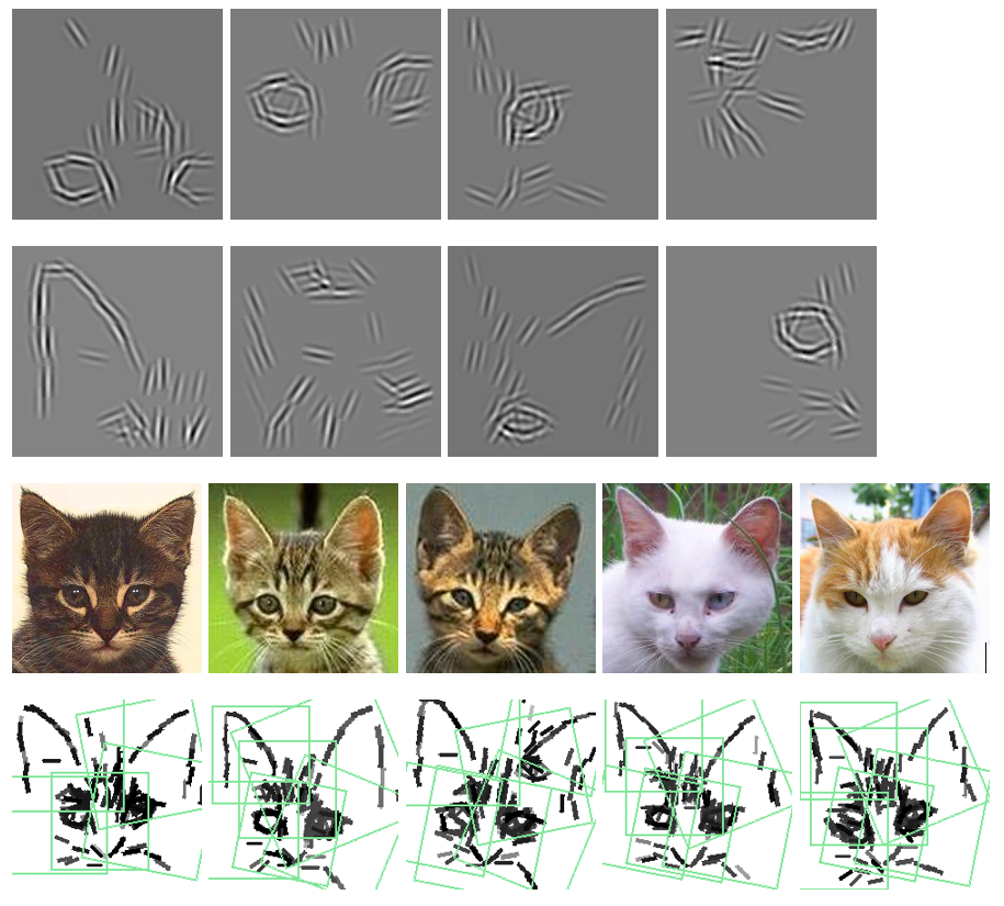
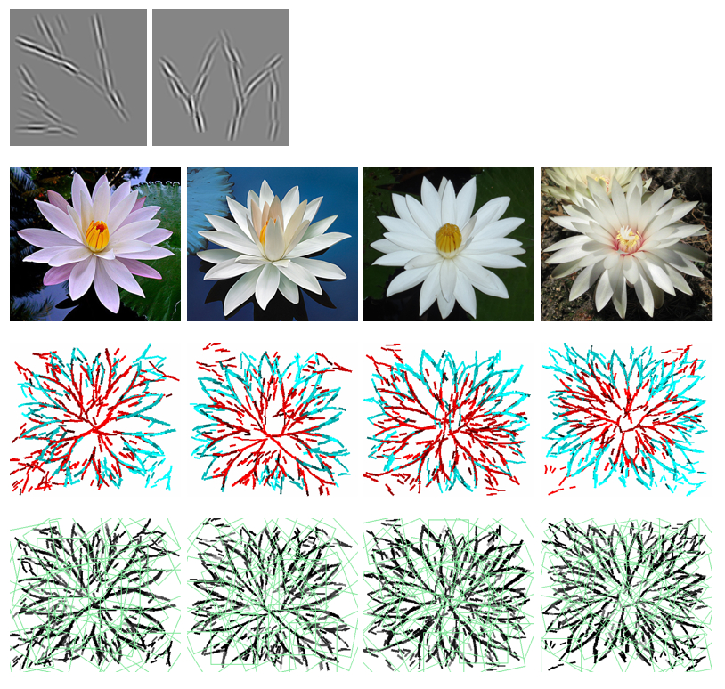
7. Unsupervised learning of codebooks
We can learn a codebook of sparse FRAME models from non-aligned images without annotation, by adopting the method of [6]. The learning algorithm iterates the following two steps: (1) Image encoding: given the current codebook, encode the training images by spatially translated, rotated, scaled versions of the models (templates) in the codebook. (2) Codebook re-learning: re-learn each model in the codebook from the image patches currently covered by this template. Figure 11 and 12 illustrate experiments of codebook learning. For the experiments in Figure 12, we select a small number wavelets of a single scale, so the synthesized images mainly capture the edge patterns.
|
|
||||
8. Object Classification Using learned Codebooks
8.1 "Bag-of-word" Representation by A Learned Codebook
The learned codebook of sparse FRAME models can serve as "words" in the "bag-of-word" method for object classification. Suppose we have a codebook of T models {B(t) , t=1, ..., T} learned from training images. For each image Im, we denote R(t)m(X,S,A)=L(Im|B(t)X,S,A) as the log-likelihood of B(t) at location X, scale S, and orientation A, both S and A are assumed to take values within a finite and properly discretized range. Let r(t)m(A)=max(maxX,S R(t)m(X,S,A), 0) be the maximum score at orientation A. Then each image Im can be represented by a T×NA-dimensional feature vector (r(t)m(A), t=1,...,T, ∀A), where NA is the number of possible values A can take. After extracting features, we can use any discriminative method to train classifiers (e.g. linear logistic regression or SVM [7]) on such feature vectors for object classification. Spatial pyramid matching (SPM) [8] can also be utilized to further boost the classification performance.
8.2 Binary Classification
|
We evaluate the "bag-of-word" representation extracted by a codebook of sparse FRAME models on a binary classification task. We test it on a collection of 16 categories from Caltech-101 [9], all 5 categories from ETHZ Shape [10] and all 3 categories from Graz-02 [11] datasets. The task is to separate each category from a negative background category. For each category, we learn a codebook of T=10 sparse FRAME templates. Each template is of the size 100 × 100 and has n = 40 wavelets. We set scale S∈{0.8, 1, 1.2} and orientation A∈{±1, 0} × π/16. Binary classification is done with linear logistic regression with regularization by l2 norm. We compare our results with those obtained by SIFT features and SVM classifier, where SIFT features are quantized into "words" by K-means clustering (K=50, 100, 500) and fed into linear or kernel SVM. The best result among these six combinations (3 numbers of words × 2 types of SVM) is then reported. Table 2 shows the comparison results of the binary classification experiments.
|
Table 2. Classification accuracies (%) on binary classification tasks for 24 categories from Caltech-101, ETHZ Shape and Graz-02 datasets
|
8.3 Multi-class Classification
Our second set of experiments is on the LHI-Animal-Faces dataset [12], which consists of around 2200 images for 20 categories of animal or human faces. We randomly select half of the images per class for training and the rest for testing. We learn a codebook of 10 sparse FRAME models for each category in an unsupervised way. We then combine the codebooks of all the categories (in total 20 × 10 = 200 codewords). The maps of the template matching scores from the models in the combined codebook are computed for each image, and they are then fed into SPM, which equally divides an image into 1, 4, 16 areas, and concatenates the maximum scores at different image areas into a feature vector. We use multi-class SVM to train image classifiers based on the feature vectors, and then evaluate the classification accuracies of these classifiers on the testing data using the one-versus-all rule. Table 3 lists four published results [12] on this dataset obtained by other methods: (a) HoG feature trained with SVM, (b) Hybrid Image Template (HIT) [12], (c) multiple transformation invariant HITs (Mixture of HIT) [12], and (d) part-based HoG feature trained with latent SVM [13]. Our method outperforms the other methods in terms of classification accuracy on this dataset.
Table 3. Classification accuracies (%) on the animal faces dataset.
HoG+SVM |
HIT |
Mixture of HIT |
Part-based LSVM |
Our method |
|---|---|---|---|---|
70.8 |
71.6 |
75.6 |
77.6 |
79.4 |
8.4 Domain Transfer
Classifiers learned from one domain (the source domain) may perform poorly on other domains (the target domains), because that training and testing data may not come from the same distribution. Learning domain-invariant feature representations can deal with this problem. In this experiment, we test our proposed representation for the task of domain transfer on four domain datasets, and compare with published results [14] [15] [16] [17] [18] [19] [20]. The four datasets are: Amazon, Webcam, DSLR and Caltech-256 [21]. Each dataset is regarded as a domain. |
Table 4. Recognition accuracies (%) on target domains (C: Caltech, A:Amazon, W:Webcam, and D:DSLR)
|
For the experiment with single source training, 10 classes common to all four datasets are extracted: backpack, touring-bike, calculator, head-phones, computer-keyboard, laptop-101, computer-monitor, computer-mouse, coffee-mug, and video-projector. For the experiment with multiple sources training, all 31 classes in Amazon, Webcam and DSLR are used. We use the evaluation protocol in [16]. |
Table 5. Performance comparison on multiple source domain transfer
|
We randomly sample labeled data in the source domain as training examples, and unlabeled data in the target domain as testing examples. We learn a combined codebook (by learning a codebook of 3 templates with n = 40 wavelets for each category and combining them together), then use it to extract feature vectors and train classifiers by multi-class SVM using the same scheme as in section 8.3. We evaluate the classification accuracies of these classifiers on the testing domain. For each pair of source and target domains, we report averaged accuracies on target domains as well as standard errors. Table 4 and Table 5 show the comparisons of recognition accuracies on target domains for single source training and multiple source training. It can be seen that our method perform significantly better than previous methods on 8 out of 11 sub-tasks, even though we do not make use of any domain adaptation techniques. This suggests that the learned codebooks of models capture intrinsically meaningful patterns.
Conclusion
The sparse FRAME model has the following properties.
(1) It can reconstruct the training images.
(2) It can synthesize new images.
(3) It separates shape deformations and appearance variations.
(4) It gives interpretable sketches.
(5) Dictionaries or codebooks of models can be learned in unsupervised manner.
(6) It combines rich traditions of harmonic analysis and Markov random field models.
References
| [1] | L. Younes. On the convergence of Markovian stochastic algorithms with rapidly decreasing ergodicity rates. Stochastics and Stochastic Reports, 65, 177-228, 1999. |
| [2] | R. Neal. MCMC using Hamiltonian dynamics. Handbook of Markov Chain Monte Carlo, 2011. |
| [3] | S. Mallat and Z. Zhang. Matching pursuit in a time-frequency dictionary. IEEE Transactions on Signal Processing, 41, 3397-3415, 1993. |
| [4] | M. Riesenhuber and T. Poggio. Hierarchical models of object recognition in cortex. Nature Neuroscience, 2, 1019–1025, 1999. |
| [5] | T. Tuytelaars, C. H. Lampert, M. B. Blaschko, and W. Buntine. Unsupervised object discovery: a comparison. IJCV, 2009. |
| [6] | Y. Hong, Z. Si, W. Hu, S.-C. Zhu, and Y. N. Wu, Unsupervised learning of compositional sparse code for natural image representation. Quarterly of Applied Mathematics, in press, 2013. |
| [7] | V. N. Vapnik. The Nature of Statistical Learning Theory. Springer, 2000. |
| [8] | S. Lazebnik, C. Schmid, and J. Ponce. Beyond bags of features: spatial pyramid matching for recognizing natural scene categories. CVPR, 2006. |
| [9] | L. Fei-Fei, R. Fergus, and P. Perona. Learning generative visual models from few training examples: an incremental Bayesian approach tested on 101 object categories. CVPR Workshop, 2004. |
| [10] | V. Ferrari, F. Jurie, and C. Schmid. From images to shape models for object detection. IJCV, 87, 284-303, 2010. |
| [11] | M. Marszalek and C. Schmid. Accurate object localization with shape masks. CVPR, 2007. |
| [12] | Z. Si and S. C. Zhu. Learning Hybrid image Template (HIT) by Information Projection. IEEE Trans. PAMI, 34, 1354–1367, 2012. |
| [13] | P. Felzenszwalb, R. Girshick, D. McAllester, and D. Ramanan. Object detection with discriminatively trained part-based models. IEEE Trans. PAMI, 32, 1627–1645, 2010. |
| [14] | K. Saenko, B. Kulis, M. Fritz, and T. Darrell. Adapting visual category models to new domains. ECCV, 213-226, 2010. |
| [15] | R. Gopalan, R. Li, and R. Chellappa. Domain adaptation for object recognition: an unsupervised approach. ICCV, 999-1006, 2011. |
| [16] | B. Gong, Y. Shi, F. Sha and K. Grauman. Geodesic flow kernel for unsupervised domain adaptation. CVPR, 2066–2073, 2012. |
| [17] | M. Yang, L. Zhang, X. Feng, and D. Zhang. Fisher discrimination dictionary learning for sparse representation. ICCV, 543-550, 2011. |
| [18] | J. Hoffman, E. Rodner, J. Donahue, K. Saenko, and T. Darrell. Efficient learning of domain-invariant image representations. ICLR, 2013. |
| [19] | S. Shekhar, V. M. Patel, H. V. Nguyen, and R. Chellappa. Generalized domain adaptive dictionaries. CVPR, 2013. |
| [20] | I. Jhou, D. Liu, D. T. Lee, and S. Chang. Robust visual domain adaptation with low-rank reconstruction. CVPR, 2168-2175, 2012. |
| [21] | G. Griffin, A. Holub, and P. Perona. Caltech-256 object category dataset. Technical report, Caltech, 2007. |
The work is supported by NSF DMS 1310391, ONR MURI N00014-10-1-0933, DARPA MSEE FA8650-11-1-7149.