Applied and Computational Harmonic Analysis
Inducing Wavelets into Random Fields via Generative Boosting
Jianwen Xie
Yang Lu
Song-Chun Zhu
Ying Nian Wu
University of California, Los Angeles (UCLA), USA
Paper | Latex | Talk
Abstract |
|
This paper proposes a learning algorithm for the random field models whose energy functions are in the form of linear combinations of rectified filter responses from subsets of wavelets selected from a given over-complete dictionary. The algorithm consists of the following two components. (1) We propose to induce the wavelets into the random field model by a generative version of the epsilon-boosting algorithm. (2) We propose to generate the synthesized images from the random field model using the Gibbs sampling on the coefficients (or responses) of the selected wavelets. We show that the proposed learning and sampling algorithms are capable of generating realistic image patterns. We also evaluate our learning method on a dataset of clustering tasks to demonstrate that the models can be learned in unsupervised setting. The learned models encode the patterns in wavelet sparse coding. Moreover, they can be mapped to the second-layer nodes of a sparsely connected convolutional neural network (CNN).
|
1. Introduction
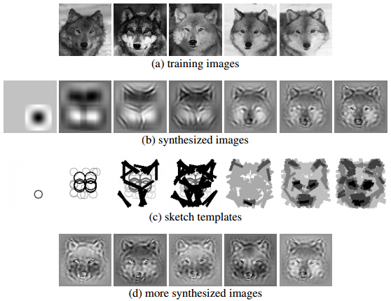
Learning Process as Painting Process. Figure 1 illustrates the learning process, which is similar to the way an artist paints a picture by sequentially fleshing out more and more details. (a) displays the training images. (b) displays the sequence of synthesized images generated by the learned model as more and more wavelets are induced into the random field by the generative boosting process. Each wavelet is like a stroke in the painting process. The wavelets are selected from a given dictionary of oriented and elongated Gabor wavelets at a dense collection of locations, orientations and scales. The dictionary also includes isotropic Difference of Gaussian (DoG) wavelets. (c) displays the sequence of sketch templates of the learned model where each selected Gabor wavelet is illustrated by a bar with the same location, orientation and length as the corresponding wavelet, and each selected DoG wavelet is illustrated by a circle (in each sketch template, wavelets of smaller scales appear darker.) (d) displays more synthesized images independently generated from the final model.
Analysis by synthesis. We synthesize images by sampling from the current model, and then select the next wavelet that reveals the most conspicuous difference between the synthesized images and the observed images. As more wavelets are added into the model, the synthesized images become more similar to the observed images. In other words, the generative model is endowed with the ability of imagination, which enables it to adjust its parameters so that its imaginations match the observations in terms of statistical properties that the model is concerned with.
|
|
Fig 1. Learning process by generative boosting. (a) observed training images (b) a sequence of synthesized images generated by the learned model as more and more wavelets are induced into the model. (c) a sequence of sketch templates that illustrate the wavelets selected from an over-complete dictionary. (d) more synthesized images. |
|
2. Past Work
Sparse FRAME and Two-stage learning. The random field model based on wavelets is called the sparse FRAME model in our previous work [1]. The model is an inhomogeneous and sparsified generalization of the original FRAME (Filters, Random field, And Maximum Entropy) model [2]. In [1], we developed a two-stage learning algorithm for the sparse FRAME model. The algorithm consists of the following two stages. Stage 1: selecting a subset of wavelets from a given dictionary by a shared sparse coding algorithm, such as shared matching pursuit. Stage 2: estimating the parameters of the model by maximum likelihood via stochastic gradient ascent where the MCMC sampling is powered by Hamiltonian Monte Carlo.
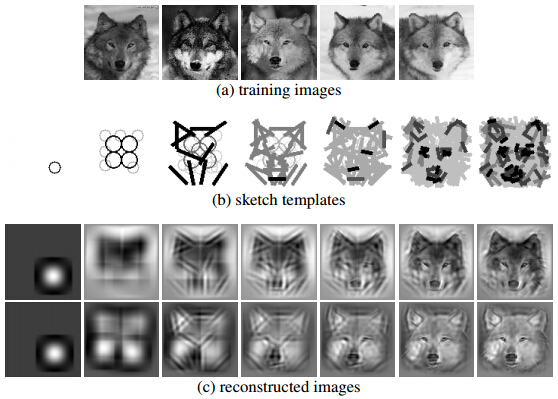
Shared Matching Pursuit. Figure 2 illustrates the shared matching pursuit algorithm. (a) displays the training images. (b) displays the sequence of sketch templates that illustrates the selected wavelets. (c) displays the sequences of reconstructed images for 2 of the 5 training images as more and more wavelets are selected by the shared matching pursuit. One conceptual concern with the two-stage learning algorithm is that the selection of the wavelets in the first stage is not guided by the log-likelihood, but by a least squares criterion that is only an approximation to the log-likelihood. In other words, the first stage seeks to reconstruct the training images by selecting wavelets, without any regard for the patterns formed by the coefficients of the selected wavelets. |
|
Fig 2. Shared matching pursuit for the purpose of wavelet selection. (a) training images. (b) sequence of sketch templates that illustrate the wavelets selected sequentially in order to reconstruct all the training images simultaneously. (c) sequence of reconstructed images by the selected wavelets for all the 1st and 3rd training images in (a). |
|
3. Random Field Models
3.1 Dense random field
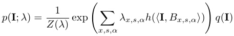
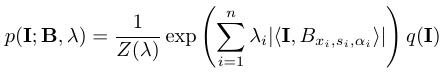
Let I be an image defined on the rectangular domain D. Let Bx,s,α denote a basis function such as Gabor wavelet (or difference of Gaussian (DoG) filter) centered at pixel x (a two-dimensional vector) and tuned to scale s and orientation α. Given a dictionary of wavelets or filer bank {Bx,s,α, ∀x,s,α} (where the scale s and the orientation α are properly discretized), the dense version of the random field model is of the following form
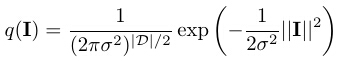
which is a Markov random field model because Bx,s,α are localized. The model is also a Gibbs distribution, an exponential family model, a log-linear model, or an energy-based model, as it is called in different contexts. In model (1), <I, Bx,s,α> is the inner product between I and Bx,s,α, or the filter response of I to the wavelet Bx,s,α. h() is a non-linear rectification function, which can be h(r) = |r|, h(r) = max(0, r), or h(r) = max(0, r-t) where t is a threshold. λ={λx,s,α, ∀x,s,α} are the weight parameters, Z(λ) is the normalizing constant, and q(I) is a white noise reference distribution whose pixel values follow independent N(0, σ2) distributions,
where ||I|| is the L2 norm of I, and D denotes the number of pixels in the image domain D. In this paper, we fix σ2=1. We normalize the training images to have marginal mean 0 and a fixed marginal variance (e.g., 10). We use h(r) = |r|, if λx,s,α > 0, then the model encourages large magnitude of the filter response <I, Bx,s,α>, regardless of its sign. This is often appropriate if we want to model object shape patterns.
3.2 Sparse random field
The dense model can be sparsified so that only a small number of are non-zero, i.e., only a small subset of wavelets is selected from the given dictionary. This leads to the following sparse model
where B=(Bxi,si,αi,i=1,...,n) are the n wavelets selected from the given dictionary, and λ=(λi, i=1,...,n) are the corresponding weight parameters.
4. Generative Boosting for Inducing Wavelets into Random Field
4.1 Generative boosting
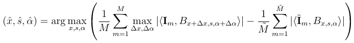
The literature on the application of boosting in learning generative models is relatively scarce. The seminal paper [3] proposed a pursuit method for inducing features into random fields. Our work can be considered a highly specialized example with a very different and specialized computational core. We propose to induce wavelets into random field by a generative version of the epsilon-boosting algorithm [4]. For notational simplicity, we use the form of dense model in equation (1), but we assume λ={λx,s,α, ∀x,s,α} is a sparse vector, i.e., only a small number of λx,s,α are non-zero. In fitting the model in (3), the algorithm starts from λ=0. Then the generative boosting algorithm updates the weight parameters λ based on the Monte Carlo estimation of the gradient. However, instead of adjusting all the weight parameters according to the gradient, the generative boosting only chooses to update the particular weight parameter that corresponds to the maximal coordinate of the gradient. Specifically, at the t-th step, we select
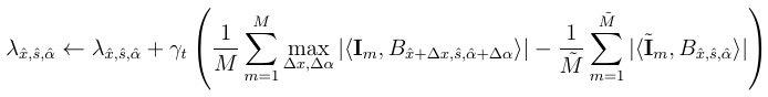
and update the corresponding weight parameter
where (Δx , Δα) are the perturbations of the location and orientation of the basis function Bx,s,α. They are introduced to account for shape deformation. { m, m = 1,...,
 } are synthesized images drawn from p(I; λ(t) ). The local max pooling is only applied to the observed images to filter out shape deformations, and we assume p(I; λ(t) ) models the images prior to shape deformations.
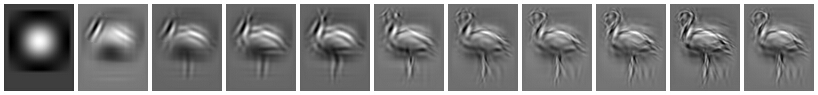
  is the step size, assumed to be a sufficiently small value. Figures 3 and Figure 4 illustrate the learning process by displaying the synthesized images generated by the learned model as more and more wavelets are included.
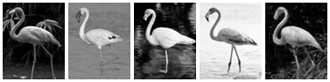
Fig 3. Learning sequence by generative epsilon-boosting (Flamingo). First row: training images. Second row: synthesized images are generated when the number of selected wavelets = 1, 40, 60, 80, 100, 200, 300, 400, 500, 600, and 700.
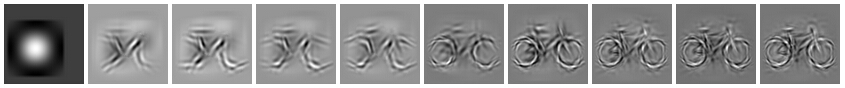
Fig 4. Learning sequence by generative epsilon-boosting (bike). First row: training images. Second row: synthesized images are generated when the number of selected wavelets = 1, 40, 60, 80, 100, 200, 300, 500, 600, and 700.
4.2 L1 solution path
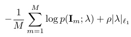
The epsilon-boosting has as interesting relationship with L1 regularization in the Lasso and the basis pursuit. As pointed out by [5], under a monotonicity condition, such an algorithm approximately traces the solution path of the L1 regularized minimization problem:
where the regulariztion parameter starts from a big value so that all the components of are zero, and gradually lowers itself to allow more components to be non-zero and to be induced the model.
4.3 Correspondence to CNN
The filer bank {Bx,s,α, ∀x,s,α} can be mapped to the first layer of Gabor-like filters of a CNN. The max∆x,∆α operations correspond to the max pooling layer. Each sparse random field model (3) can be mapped to a node in the second layer of a CNN, where each second layer node is sparsely and selectively connected to the nodes of the first layer, with λi being the connection weights. The generative boosting algorithm is used to sparsely wire the connections. − log Z(λ) can be mapped to the bias term of the second-layer node.
5. Gibbs Sampler on Wavelets Coefficients
5.1 Wavelet sparse coding
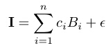
In order to power the generative boosting algorithm, we need to sample from the currently learned model. We develop a Gibbs sampling algorithm that generates the synthesized images by exploiting the generative form of the model. The sparse model in equation (3) can be translated into a generative model where the selected wavelets serve as linear basis functions. Given the selected basis functionsB=(Bi=Bxi,si,αi,i=1,...,n), we can represent the image I by
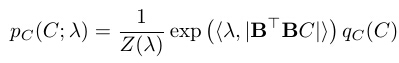
where ci are the least squares reconstruction coefficients, and Ɛ is the residual image after we project I onto the subspace spanned by B. We can write I, Bi, and C as column vectors, so that B=(Bi, i=1,...,n) is a matrix. It can be shown that under the model p(I; B, λ) in (3), the distribution of C is
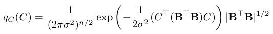
where
is a multivariate Gaussian distribution, i.e., under qC(C), C ~ N(0, σ2(BTB)-1). The notation | • | is the operation taking element-wise absolute values.
5.2 Moving along basis vectors
For Gibbs sampling of C~qC(C; λ), an equivalent but simpler way of updating the i-th component is by first sampling from
and let
where di is a scalar increment of ci. The change from I to I+di Bi only changes ci while the other coefficients remained fixed. So this scheme implements the same move as the update in the Gibbs sampler.
6. Synthesis by Generative Boosting
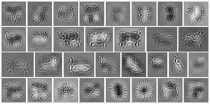
Figure 5 displays some images generated by the sparse random field models, which are learned by the generative epsilon-boosting from roughly aligned images. The proposed learning algorithm is capable of modeling a wide variety of image patterns.
|
|
Fig 5. Synthesis by generative boosting. Images generated by the random field models learned from different categories of objects. Typical size of the images are 100x100. Typical number of training images for each category is around 5. Number of the selected wavelets is 700. |
|
References
| [1] |
Xie, J., Hu, W., Zhu, S. C., & Wu, Y. N. Learning Sparse FRAME Models for Natural Image Patterns. International Journal of Computer Vision, 114(2-3), 91-112, 2015 |
| [2] |
Zhu, S. C., Wu, Y. N., & Mumford, D. Minimax entropy principle and its application to texture modeling. Neural computation, 9(8), 1627-1660, 1997 |
| [3] |
Stephen Della Pietra, Vincent Della Pietra, and John Lafferty. Inducing features of random fields. Pattern Analysis and Machine Intelligence, IEEE Transactions on, 19(4):380–393, 1997 |
| [4] |
Jerome H Friedman. Greedy function approximation: a gradient boosting machine. Annals of Statistics, 29(5):1189–1232, 2001.
|
| [5] |
Saharon Rosset, Ji Zhu, and Trevor Hastie. Boosting as a regularized path to a maximum margin classifier. The Journal of Machine Learning Research, 5:941–973, 2004. |
The work is supported by NSF DMS 1310391, ONR MURI N00014-10-1-0933, DARPA MSEE FA8650-11-1-7149.