Active Basis Model
 ,
Shared Sketch Algorithm
,
Shared Sketch Algorithm
 ,
and Sum-Max Maps
for Representing, Learning, and Recognizing Deformable Templates
,
and Sum-Max Maps
for Representing, Learning, and Recognizing Deformable Templates
Ying Nian Wu, Zhangzhang Si, Haifeng Gong, and Song-Chun Zhu

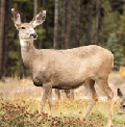
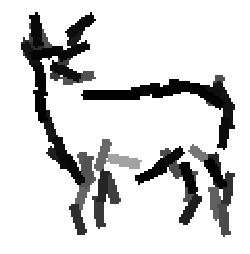
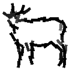
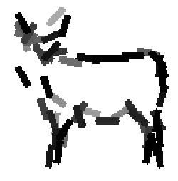
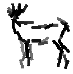
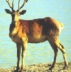
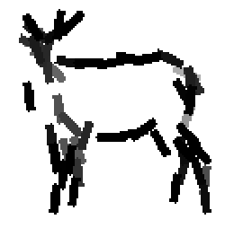
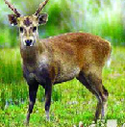
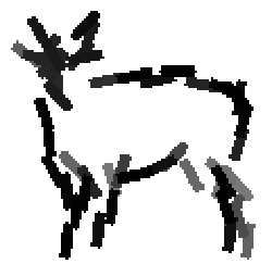
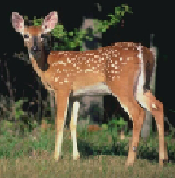
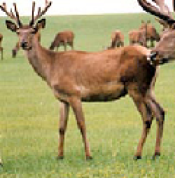
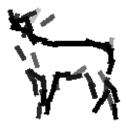
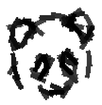
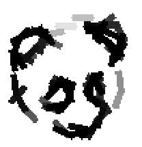
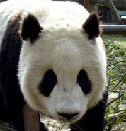
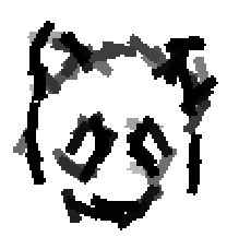
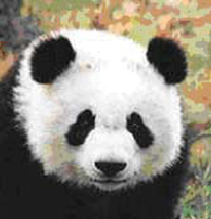
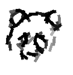
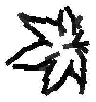
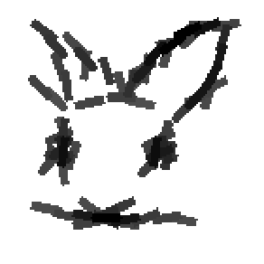
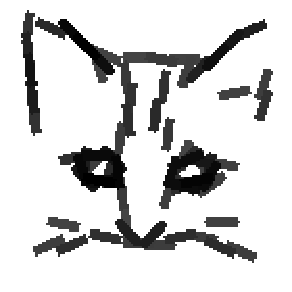
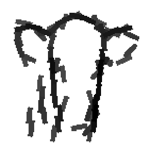
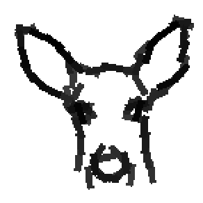
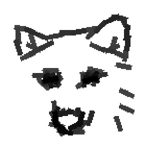
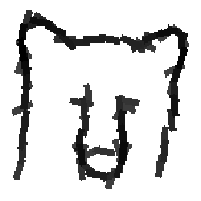
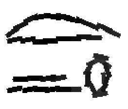
Learning the template from the training images. Each selected Gabor basis
element is represented by a bar.
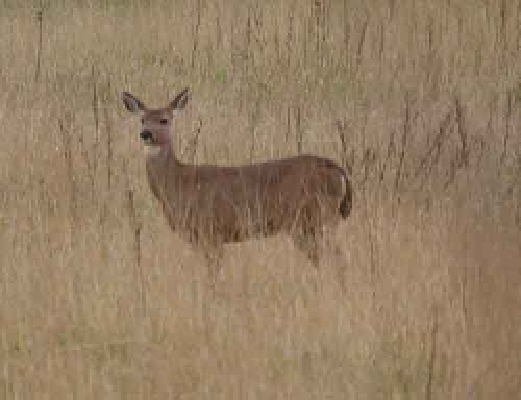
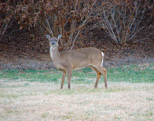
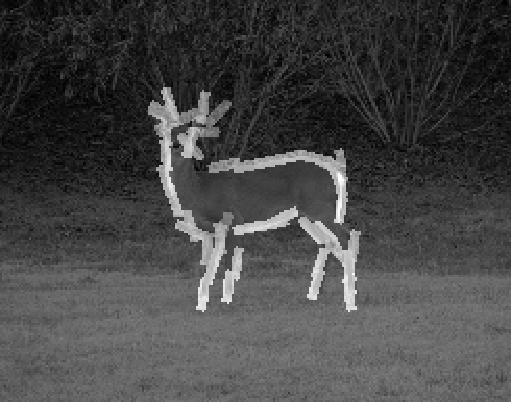
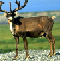
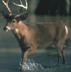
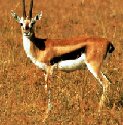
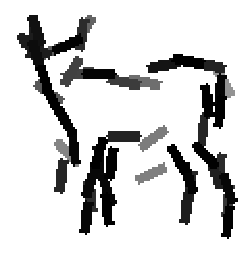
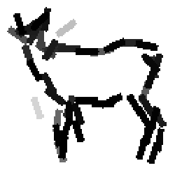
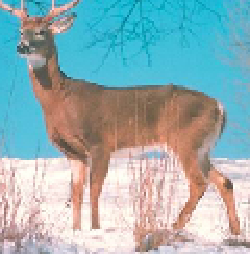
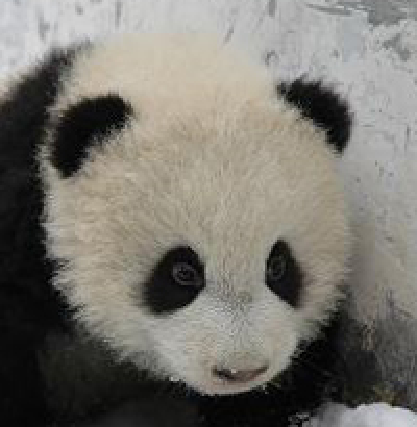
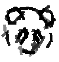
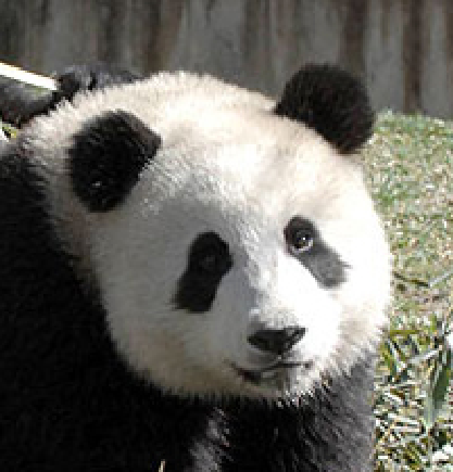
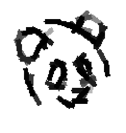
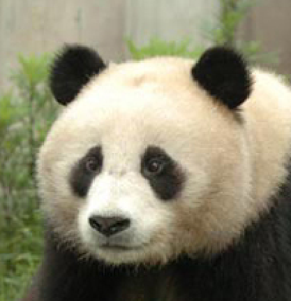
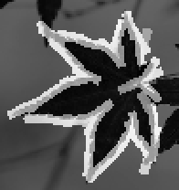
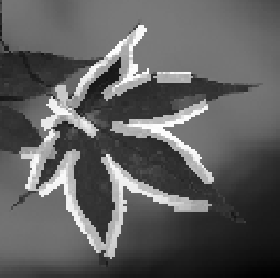
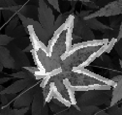
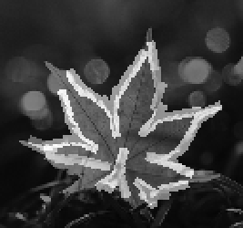
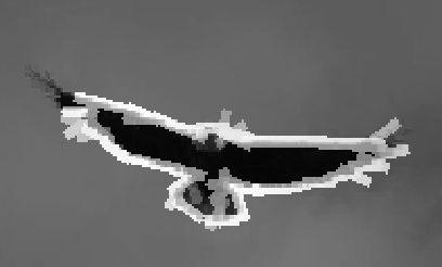
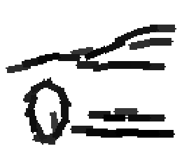
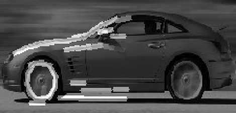
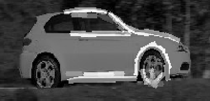
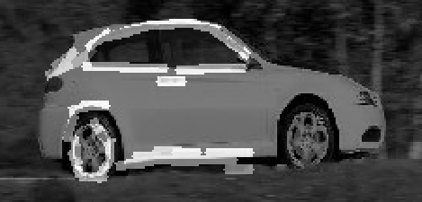
Detecting and sketching the objects in the testing images using
the learned template.
Examples of learning and detecting cats.


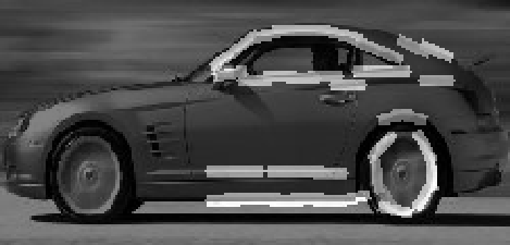
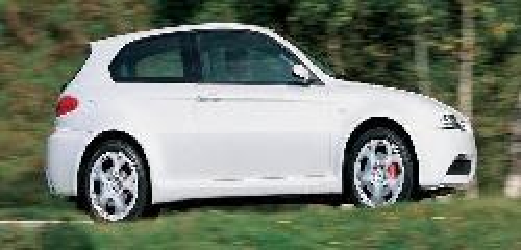
Allowing uncertainties in locations, scales and orientations of objects in training data.
 |
|
 |
|


Finding clusters in mixed training data.


Learning part templates for finer sketch at higher resolution.
Paper |
Code |
Experiments |
Model |
Learning |
Inference |
Hierarchical |
Texture
The code in this section is more readable and up-to-date than the code in
Section 3. You can start reading from the file "ReadMeFirst".
Typical parameters: scale parameter of Gabor = .7; locationShiftLimit = 4 pixels
(reduced to 3 pixels if it is allowed to adjust overall locations, scales and rotations as in 2);
The length or width of the bounding box is around 100 pixels. For larger scale (e.g., scale parameter = 1), you can change
locationShiftLimit and the size of bounding box proportionally. You can tune these parameters, although
in principle they can be selected automatically.
- Learning from roughly aligned images and detection using learned template.
(a)
Basic version
This code is the basis for other code. It learns single-scale template in the learning step. It searches over multiple resolutions, rotations and
left-right poses in the inference (detection, recognition) step. The learning step and the inference step are usually iterated in an
unsupervised learning algorithm. The active basis model is designed for unsupervised learning, such as the learning of codebooks.
(b) Local shift version
Recommended.
It learns single-scale template. It allows local shift in location, scale, rotation as well
as left-right flip of the object in each training image.
- Learning from images where the locations, scales, orientations and left-right poses
of the objects are unknown.
Basic version It learns single-scale template.
It searches over multiple resolutions, rotations and
left-right poses in detection.
- Clustering by fitting a mixture of active basis models.
(a)
Basic EM version It learns single-scale templates.
It is initialized by random clustering, with rigorous implementation of E-step. This code only serves as a proof of concept.
(b)
Local shift version Recommended.
It searches over multiple resolutions, rotations and
left-right poses in detection. It starts from random clustering, and allows for multiple starting.
- Learning multi-scale templates.
(a)
Learning from aligned images This code has a different structure and embellished
features. It learns templates at multiple scales. It uses Gabor wavelets at multiple scales, although
one can also use single-scale Gabor wavelet and multiple resolutions of images.
(b)
Learning from non-aligned images Based on the code in 4.(a)
Post-pulication experiences
- Discriminative adjustment by logistic regression: Conditioning on
hidden variables, the active basis model implies a logistic regression for
classification based on MAX1 scores of the selected basis elements.
The lambda parameters of the active basis
model can be re-estimated discriminatively by regularized logistic regression
to further improve classification performance. See
Experiment 16
done by Ruixun Zhang, then
a summer visiting student from Peking U.
- Model-based clustering: The EM algorithm for clustering with random initialization seems to perform better
than we claimed in the paper, if the number of training examples in each cluster is
not too small.
See Experiment 17.
- Local normalization: We have experimented with local normalization of
filter responses (e.g., scale parameter = .7, half window size = 20), which
is the option (3) in section 3.5 of the paper. We have posted the code and results in the experiments pages
in Section 3. It appears that local normalization is better than normalization within
the template window, i.e., the option (2) in section 3.5 of the paper, in terms of
the appearances of the learned templates and the classification performances.
The local normalization is also easier to implement than normalization within the
template window. In the updated code of Section 2, we have enforced this option as the only
option for normalization.
- Range of activity: We have also experimented with reduced range of activity (e.g., up to 3
or 4 pixels, where subsampling rate is 1). The model is still quite resilient with reduced
activity, which gives tighter fit. For cleaner template, it is important to resize the images to a proper size,
so that the bounding box of the template is not too large, e.g., around 100 pixels. In principle, finding the
right template size can be done automatically by maximum likelihood.
- Saturation level: The current saturation level in the sigmoid transformation is 6 (after
local normalization). Experiments on classification suggest that the performance is optimal if it is
lowered to 3.5. It is still unclear whether this level is better for unsupervised learning.
The section includes some experiments done after the publication of the two technical reports.
- The code in this section is only for reproducing the experiments. We deliberately
keep some fossilized versions of the code in this section for our own record. See
Section 2 for the most updated code.
- In the mex-C-code "Clearn.c" in this Section 3, many lines are devoted to a bin-chain trick
for global maximization during learning. It now appears that this trick does not speed up the
computation very much, unless the images are very large. So in the updated code in Section 2,
we do not use this trick.
- We also posted code where we normalize each filter
response by the local average within a local window, by or the average response within the
scanning window of the template.
- For most experiments, we also posted code where we use two large natural images as
background images to pool the marginal distributions of filter responses.
There is no much change in results.
- The experiments are re-numbered in the revised version of the manuscript.
-
Experiments 1 and 2
Supervised learning (without local shift) and detection
ETHZ shape data
Supervised learning (without local shift)
LHI data of animal faces etc.
Supervised learning with local shift which improves learning results ( 25 experiments )
- Experiment 3
Supervised learning and classification
- Experiment 4
Model-based clustering (without local shift)
- Experiment 5
Learning from non-aligned images with unknown locations and scales, but the same
rotation and aspect ratio
- Experiment 6
Learning moving template
- Experiment 7
Composing multiple templates
- Experiment 8
Geometric transformation of template
- Experiment 9
Local learning of representative templates
- Experiment 10
Synthesis by multi-scale Gabors and DoGs
- Experiment 11
Clustering initialized by local learning
- Experiment 12
Discriminative learning by adaboost
- Experiment 13
Learning with unknown rotations plus unknown locations and scales and left-right flip
(100+ experiments on learning patterns of natural scenes)
- Experiment 14
Composing simple geometric shapes into shape scripts
- Experiment 15
Learning hierarchical active basis by composing partial templates
- Experiment 16
Discriminatively adjusting active basis model by regularized logistic regression
(summer project of Ruixun Zhang, then a visiting
undergraduate student from Peking U)
- Experiment 17
Model-based clustering while allowing local shifts of templates
Bug reports
We did not clean the bugs from all the code in the above experiments,
because they do not affect the existing results.
Version cross-validation
Check the code by comparing different versions or implementations.
How to represent a deformable template?
The answer is no much beyond wavelet representation, just add some perturbations
to the wavelet elements.
The perturbations and the coefficients of the wavelet elements
are the hidden variables that seek to explain each individual training image.
Active basis. Each Gabor wavelet element is illustrated by a thin ellipsoid at a certain
location and orientation. The upper half shows the perturbation of one basis element.
By shifting its location or orientation or both within a limited range, the basis
element (illustrated by a black ellipsoid) can change to other Gabor wavelet
elements (illustrated by the blue ellipsoids). Because of the perturbations of the
basis elements, the active basis represents a deformable template.
eps
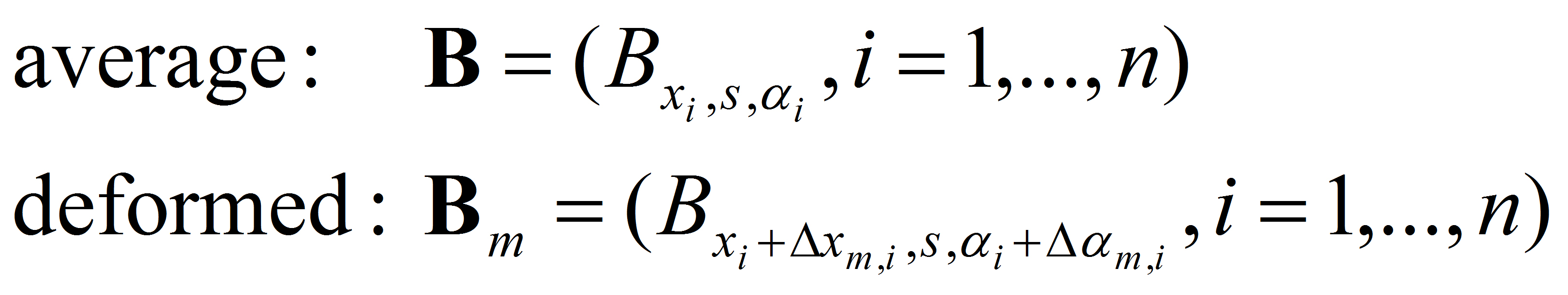
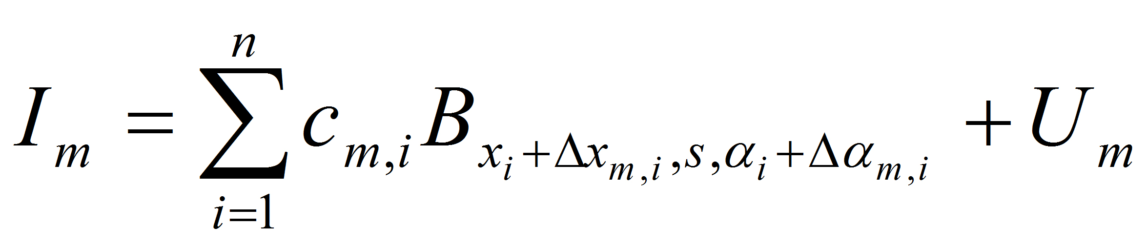
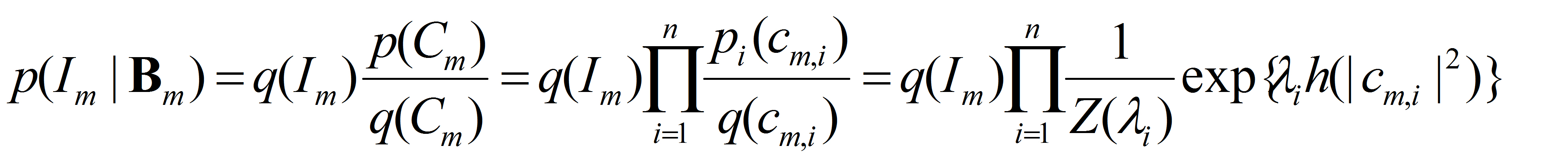
whew "I" stands for training image, "B" stands for basis, "c" stands for coefficients, "x" stands for
pixel, "s" stands for scale, "alpha" stands for orientation, "i" indexes
basis elements, "m" indexes training images, "Delta" stands for perturbations
or activities. The Delta x and Delta alpha are hidden variables that are to be inferred.
Simplicity: the active basis model is a simplest generalization of the Olshausen-Field V1 model,
and we hope it may be relevant to the cortex beyond V1.
The generalization is in the subscripts (or attributes).
The model is also a simplest instance of AND-OR graph advocated by Zhu and Mumford for vision. AND means composition of basis elements,
OR means variations of basis elements caused by Detla hidden variables. The Delta variables can be understood as "residuals" of
a shape model built on the geometric attributes of basis elements, where the shape model takes the form of an average shape plus residuals,
which is the simplest shape model.
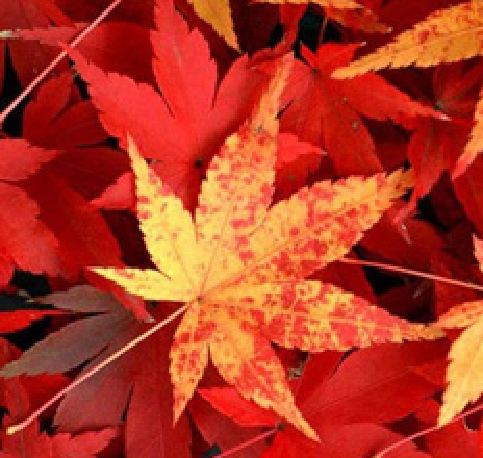
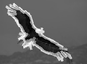
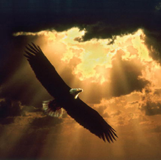
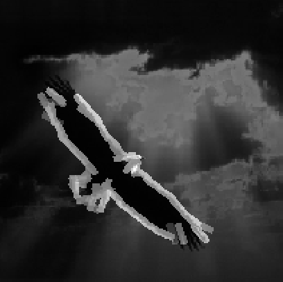
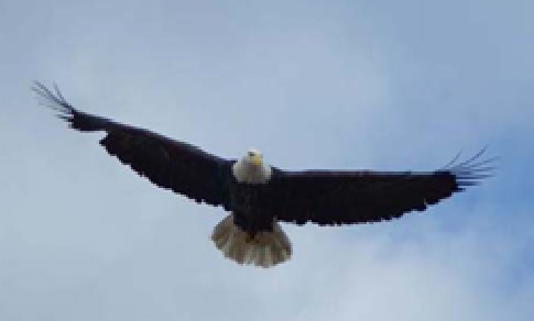
The following are the deformed templates matched to the training images. They are not
about motion. They illustrate deformations.


The model is generative and seeks to explain the images.
The probability model at the bottom layer, i.e., conditioning on the Delta hidden variables or equivalently the deformed template B_m, is
How to learn a deformable template from a set of training images?
The answer is no much beyond matching pursuit, just do it simultaneously on
all the training images.
The intuitive concepts of "edges" and "sketch" emerge from this process.
Shared sketch algorithm. A selected element (colored ellipsoid) is shared by all the
training images. For each image, a perturbed version of the element seeks
to sketch a local edge segment near the element by a local maximization operation.
The elements of the active basis are selected sequentially according to the
Kullback-Leibler divergence between the pooled distribution (colored solid curve)
of filter responses and the background distribution (black dotted curve).
The divergence can be simplified into a pursuit index, which is the sum of
the transformed filter responses. The sum essentially counts the number of
edge segments sketched by the perturbed versions of the element.
eps
 The prototype of the algorithm is the shared matching pursuit algorithm:
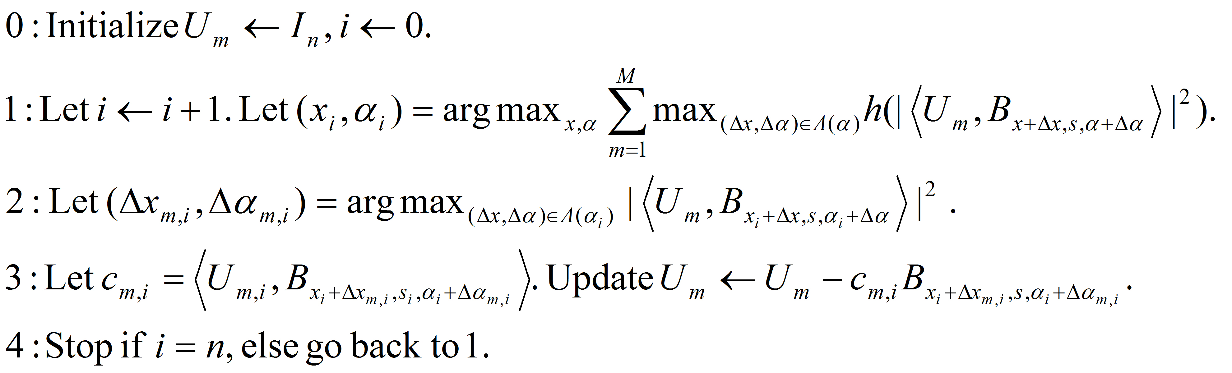
The generative learning is largely defined by Step (3), which is matching pursuit
explaining away, and which leads to non-maximum suppression performed separately on each individual image.
After learning the deformable template, how to recognize it in a new image?
The answer is no much beyond Gabor filtering, just add a local max filtering,
and then a linear shape filtering.
But this is to be followed by a top-down pass
for sketching the detected object.
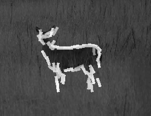
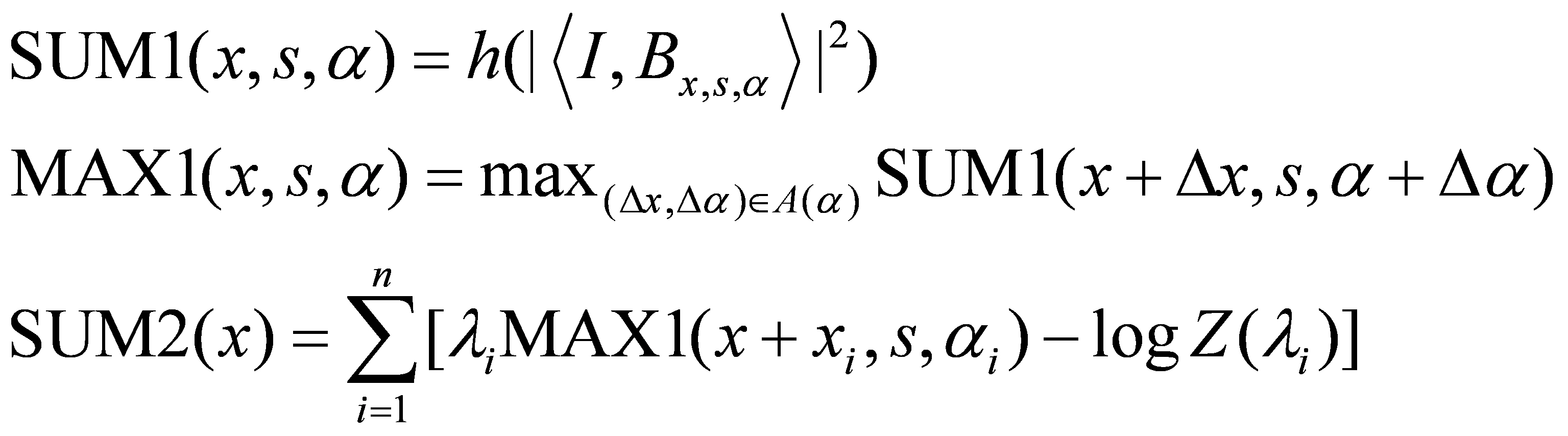
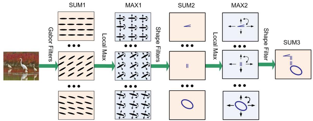
Sum-max maps. The SUM1 maps are obtained by convolving the input image with Gabor
filters at all the locations and orientations. The ellipsoids in the SUM1 maps
illustrate the local filtering or summation operation. The MAX1 maps are obtained
by applying a local maximization operator to the SUM1 maps. The arrows in the
MAX1 maps illustrate the perturbations over which the local maximization is taken.
The SUM2 maps are computed by applying a local summation operator to the MAX1 maps,
where the summation is over the elements of the active basis. This operation
computes the log-likelihood of the deformed active basis, and can be interpreted
as a shape filter.
The bottom up process computes the log-likelihood
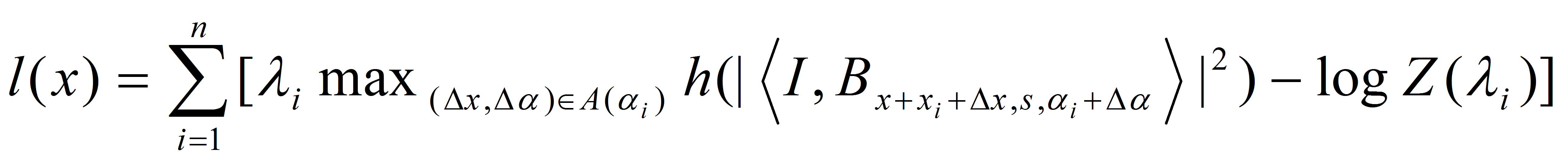
It can be decomposed into the following bottom-up operations:
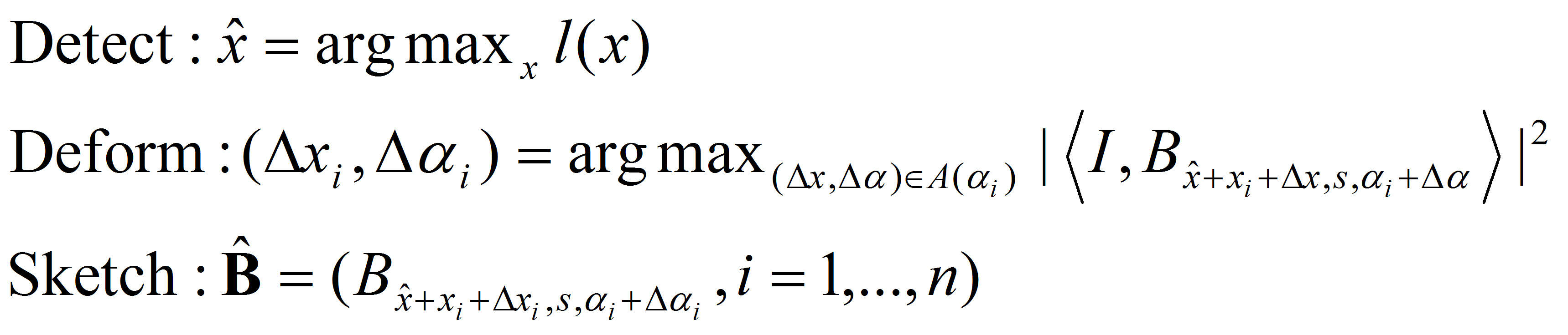
which are followed by the following top-down operations:
The above architecture is more representational than operational, more top-down than
bottom-up. The bottom-up operation serves the purpose of top-down representation.
The neurons in MAX1 layer can be interpreted as representational OR-nodes of AND-OR graph, where
max operation in bottom-up serves the purpose of arg-max inference in top-down.
The neurons in SUM2 layer represent templates or partial templates by selective
connections to neurons in MAX1 layer.
How to model more articulated objects?
The answer is to further compose multiple active basis models that serve as part-templates.
The hierarchical model and the inference architecture are recursions of the themes in active basis.
Sum-max maps. A SUM2 map is computed for each sub-template. For each SUM2 map,
a MAX2 map is computed by applying a local maximization operator to the SUM2 map.
Then a SUM3 map is computed by summing over the two MAX2 maps. The SUM3 map
scores the template matching, where the template consists of two sub-templates
that are allowed to locally shift their locations.
eps
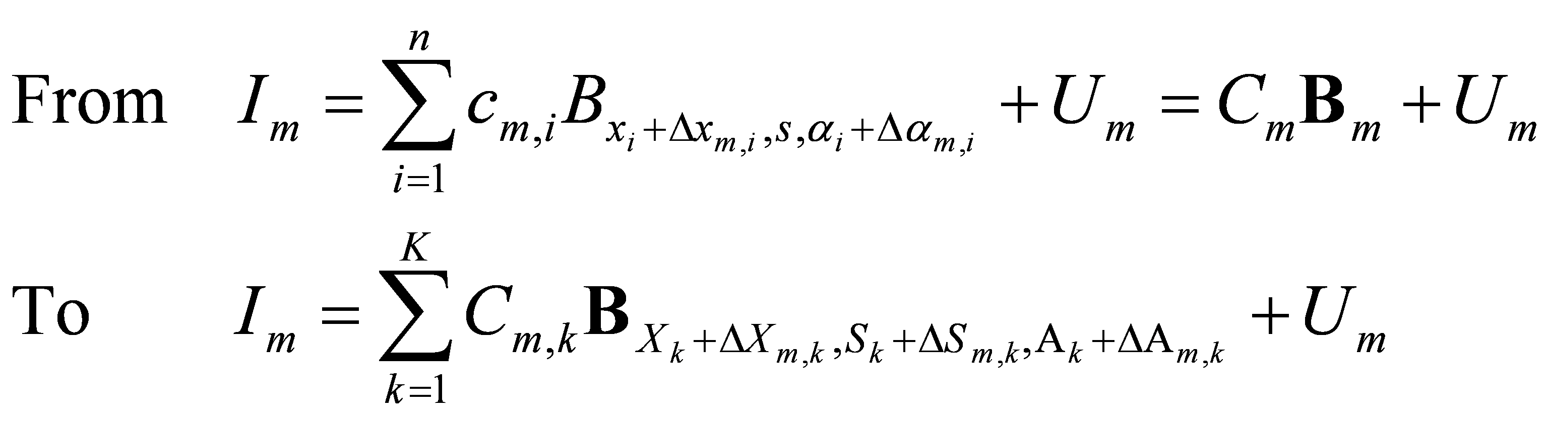
The hierarchical
active basis model shares the same form as the original active basis model.
Shape Script Model
Composing simple geometric shapes (line segments, curve segments,
parallel bars, angles, corners, ellipsoids) represented by active basis models.
Are they related to V2 cells or beyond?
Sum-max maps. The sub-templates can be simple geometric shapes describable by simple geometric attributes,
such as line segments, curve segments,
corners, angles, parallels, ellipsoids, that are allowed to change their attributes such as locations, scales,
orientations, as well as aspect ratios, curvatures, angles etc.
Where do texture statistics come from?
The answer is that they are pooled as null hypothesis to test the sketch hypothesis.
The null hypothesis itself also provides strong description of image intensity pattern.
Nonadaptive background (or negative) images. The residual image of the active basis
model is assumed to share the same marginal statistics as these images.
 eps
eps
 eps
eps
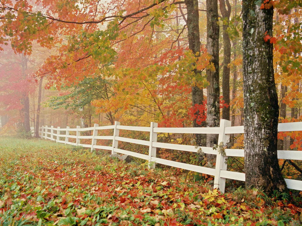
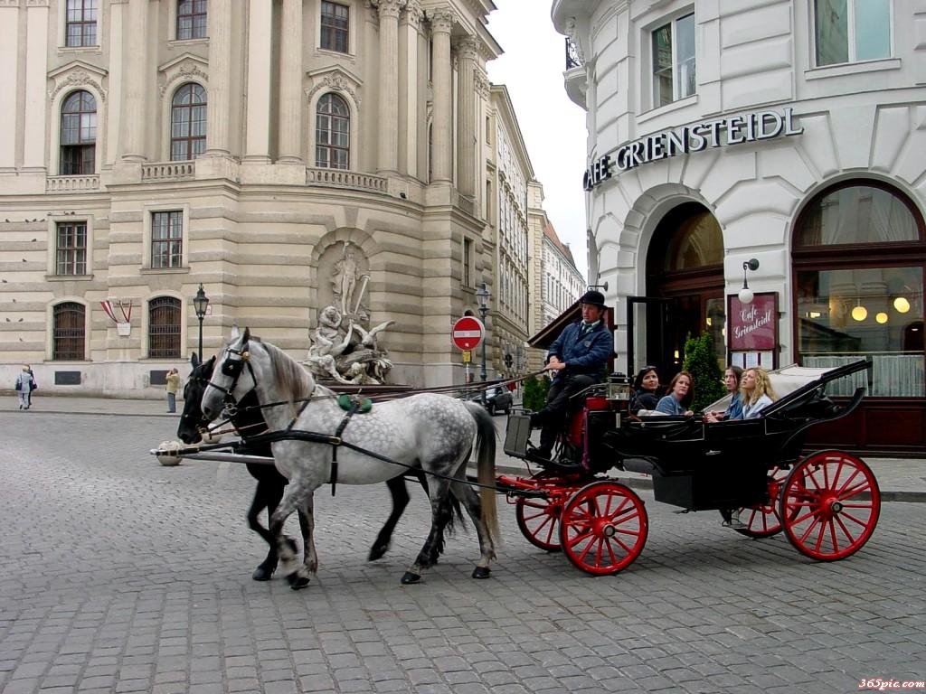
Both images are 1024x768. The left image is a rural scene (higher entropy and lower kurtosis),
and the right image is an urban scene (lower entropy and higher kurtosis).
 eps
eps
 eps
eps
 eps
eps
Left: Marginal density q() of responses pooled from the above two natural images.
It is roughly invariant over scales of Gabor wavelets. It has a very long tail
(the small bump at the end is caused by sigmoid saturation), reflecting the
fact that there are edges in natural images. The densities of the active basis
coefficients are exponential tilting of q().
Middle: Link function between natural parameter and mean parameter. This is used
to infer the natural parameters from the observed mean responses at selected
locations and orientations.
Right: Log of normalizing constant versus natural parameter. This is used for
calculating log-likelihood ratio score for template matching.
Adapative background, where the marginal density q() is pooled from testing images directly.
 eps
eps
For each image, at each orientation, a marginal histogram q of filter
responses is pooled over all the pixels of this image. Such adaptive q forms a natural couple
with p, so that their ratios can be used to score template matching. Such marginal
histograms lead to the
Markov random
field model of texture. The concept of stochastic texture arises as a summary
of failed sketching, or as the strongest null hypothesis against the hypothesis of
sketchability.
The explicit form of the Markov random field texture model is
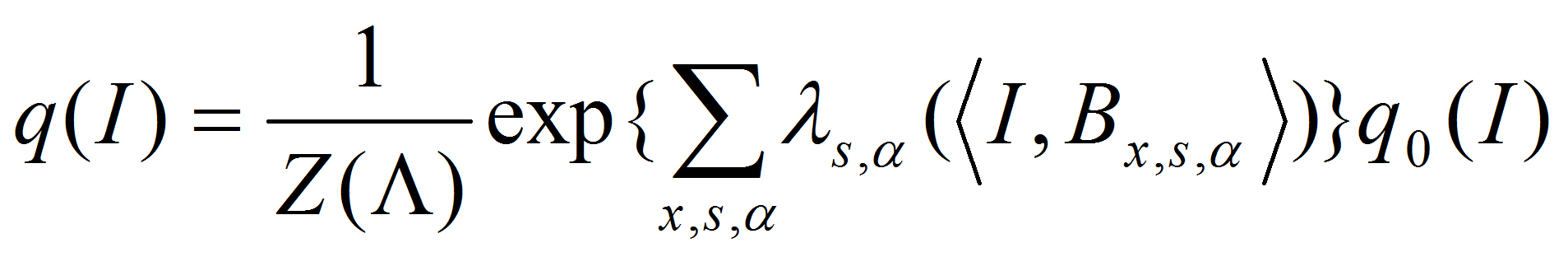
Paper |
Code |
Experiments |
Model |
Learning |
Inference |
Hierarchical |
Texture
Research reported on this page has been supported by
NSF DMS 0707055, 1007889 and NSF IIS 0713652.
Back to active basis homepage